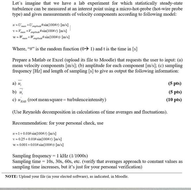
Let's imagine that we have a lab experiment for which statistically steady-state turbulence can be measured at an interest point using a micro-hot-probe (hot-wire probe type) and gives measurements of velocity components according to following model: u=U +U V&V +V WW +W man m #sin(100#r) [m/s] #sin(100#7) [m/s] #sin(100#t) [m/s] Where, "#" is the random function (0 1) and t is the time in [s] Prepare a Matlab or Excel (upload its file to Moodle) that requests the user to input: (a) mean velocity components [m/s]; (b) amplitude for each component [m/s]; (c) sampling frequency [Hz] and length of sampling [s] to give as output the following information: a) u, b) 11, c) RMS (root mean square= turbulence intensity) (5 pts) (5 pts) (10 pts) (Use Reynolds decomposition in calculations of time averages and fluctuations). Recommendation: for your personal check, use u=1+0.01# sin(100# r) [m/s] v 0.25 +0.01# sin(100#r) [m/s] w = 0.001 +0.01# sin(100# r) [m/s] Sampling frequency = 1 kHz (1/1000s) Sampling time = 10s, 30s, 60s, etc. (verify that averages approach to constant values as sampling time increases, but it's just for your personal verification) NOTE: Upload your file (in your elected software), as indicated, in Moodle.