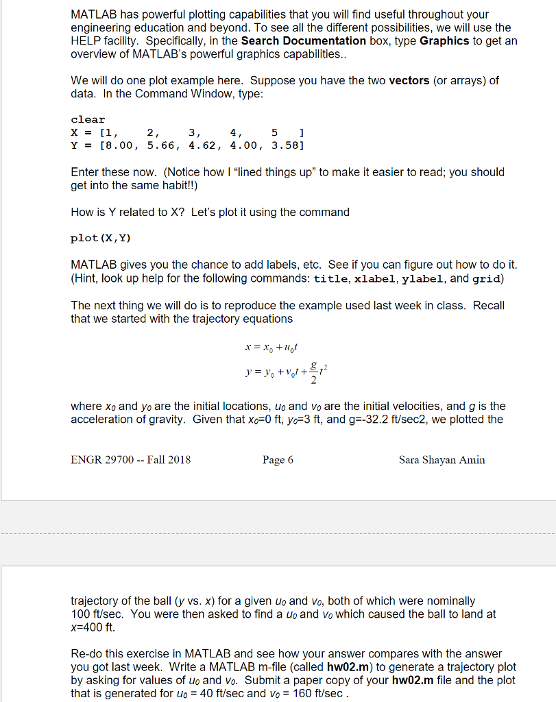
MATLAB has powerful plotting capabilities that you will find useful throughout your engineering education and beyond. To see all the different possibilities, we will use the HELP facility. Specifically, in the Search Documentation box, type Graphics to get an overview of MATLAB's powerful graphics capabilities We will do one plot example here. Suppose you have the two vectors (or arrays) of data. In the Command Window, type cllear 2 3 Y= [8.00, 5.66, 4.62, 4.00, 3.58] Enter these now. (Notice how | "lined things up" to make it easier to read; you should get into the same habit!!) How is Y related to X? Let's plot it using the command plot (X, Y) MATLAB gives you the chance to add labels, etc. See if you can figure out how to do it. (Hint, look up help for the following commands: title, xlabel, ylabel, and grid) The next thing we will do is to reproduce the example used last week in class. Recall that we started with the trajectory equations where xo and yo are the initial locations, uo and vo are the initial velocities, and g is the acceleration of gravity. Given that xo-0 ft, yo-3 ft, and g-32.2 ft/sec2, we plotted the ENGR 29700 - Fall 2018 Page 6 Sara Shayan Amin trajectory of the ball (y vs. x) for a given uo and vo, both of which were nominally 100 ft/sec. You were then asked to find a uo and Vo which caused the ball to land at x 400 ft. Re-do this exercise in MATLAB and see how your answer compares with the answer you got last week. Write a MATLAB m-file (called hw02.m) to generate a trajectory plot by asking for values of uo and vo. Submit a paper copy of your hw02.m file and the plot that is generated for uo = 40 ft/sec and Vo = 160 ft/sec