Matlab help

Here's the code from exercise 2 : (Please finish the ex3 which will use the code from ex2 and paste the code clearly)

f=@(t,y) 1-exp(-4*t)-2*y

[T,Y]=ode45(f,[0,3],2);

hold on;

plot(T,Y,'+g');

plot(T,Y,'r')

Here's the code of Code Snippet 1

% Interval bounds

tmin =0;

tmax =3;

ymin=0;

ymax=2;

% Grid spacing

spacing = 0.3;

% Define x and y coordinates

[pt , py] = meshgrid(tmin:spacing:tmax,ymin:spacing:ymax);

% Calculate slopes

ydash = 1-exp(-4*pt)-2*py;

% Define slope vector components

dt = (spacing/2)./sqrt(1+ydash.^2);

dy = ydash.*dt;

% Clear the figure

clf;

% Create slope field

q = quiver(pt, py, dt, dy,'b','AutoScale','off');

set(q,'ShowArrowHead','off','LineWidth',1)

% Set axis and labels

axis([tmin tmax ymin ymax])

xlabel('x')

ylabel('y')

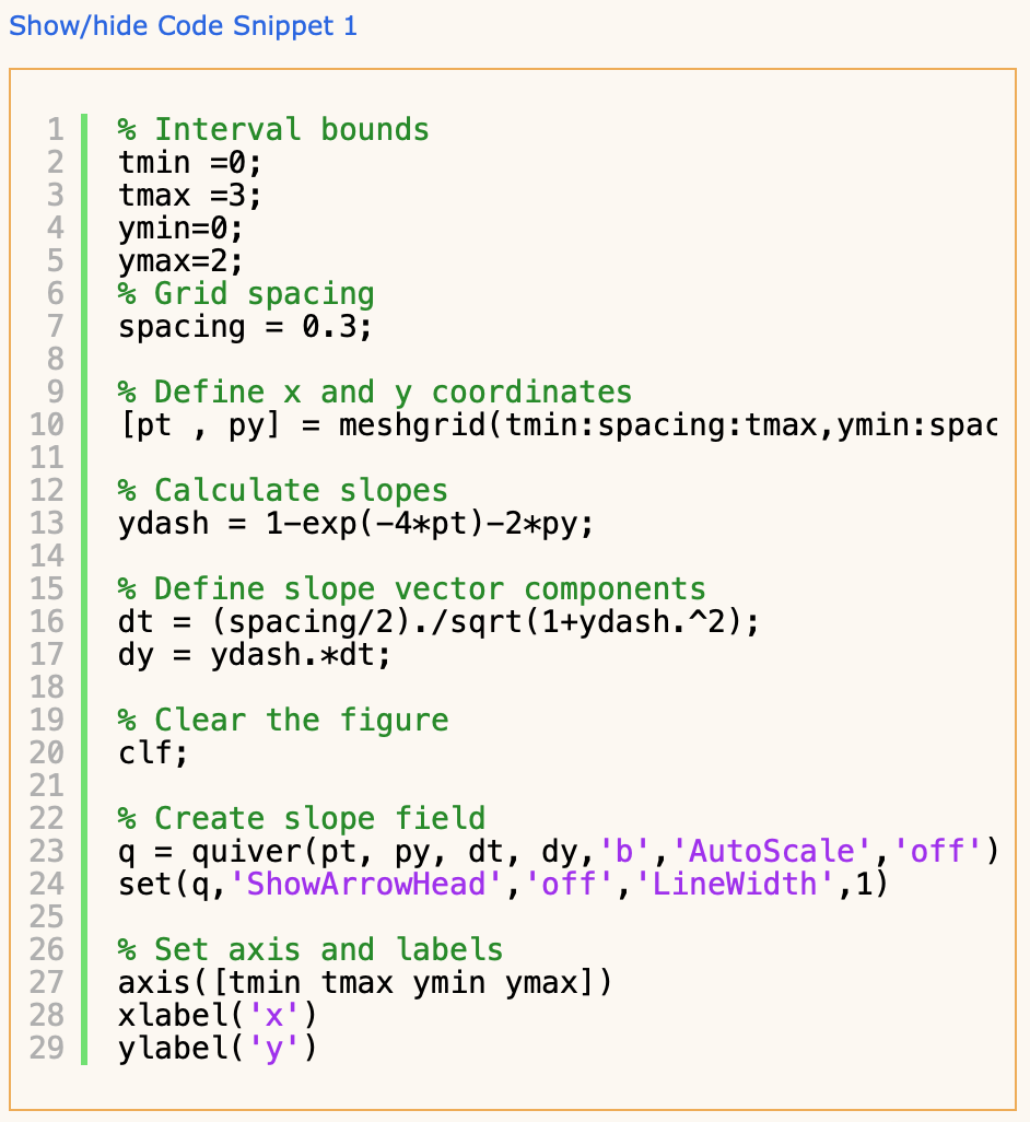
Exercise 3 The following code snippet will produce a slope field for the ODE dy di = f(t,y), y(0) = 2, Osts3 where f(t, y) = 1 e-44 2y. Show/hide Code Snippet 1 HNMONOO OOHNM % Interval bounds tmin =0; tmax =3; ymin=0; ymax=2; % Grid spacing spacing = 0.3; % Define x and y coordinates [pt , py] = meshgrid(tmin: spacing: tmax, ymin: spac % Calculate slopes ydash = l-exp(-4*pt)-2*py; % Define slope vector components dt = (spacing/2)./sqrt(1+ydash.^2); dy = ydash.*dt; 10 11 12. 13 14 15 16 17 18 19 20 21 22 23 24 25 26 27 28 29 % Clear the figure clf; % Create slope field q = quiver(pt, py, dt, dy, 'b', 'AutoScale','off') set(q, 'ShowArrowhead','off', 'LineWidth',1) % Set axis and labels axis ( [tmin tmax ymin ymax]) xlabel('x'). ylabel('y'). Run Code Snippet 1 and by adapting your answers from Exercise 2, plot a numerically approximated solution to the IVP over the top of the slope field. Save your figure as a PNG image and submit using the following prompt. Show/hide tip on saving as a PNG To save the current figure as a PNG you can use the command: print("module10.png','-dpng') or simply select Save As... from the Figure Window. But be careful! Make sure you select the .png file type when you save your figure. Choose File no file selected Upload your PNG 0% From looking at your plot do you think the numerically approximated solution is accurate? Explain. Enter