matlab

it is provided

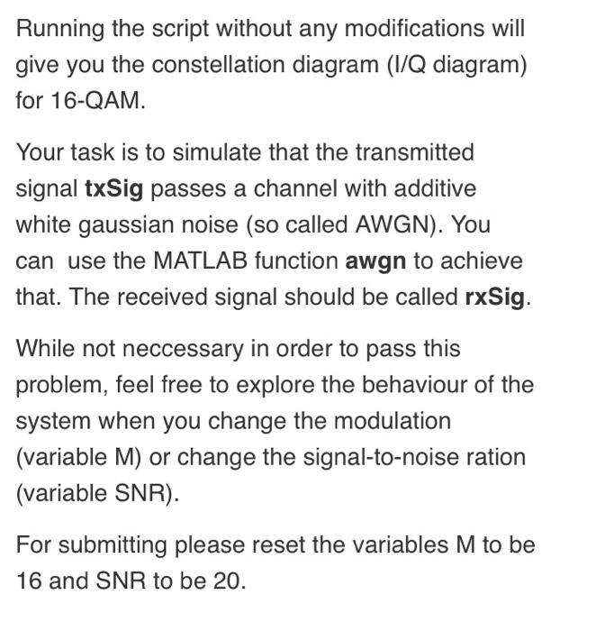
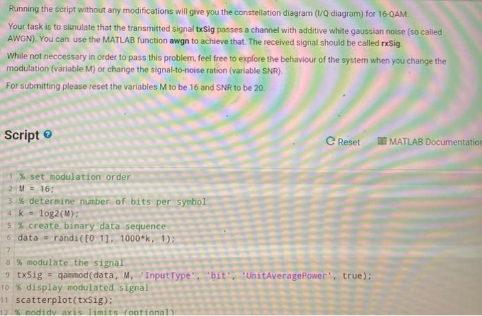
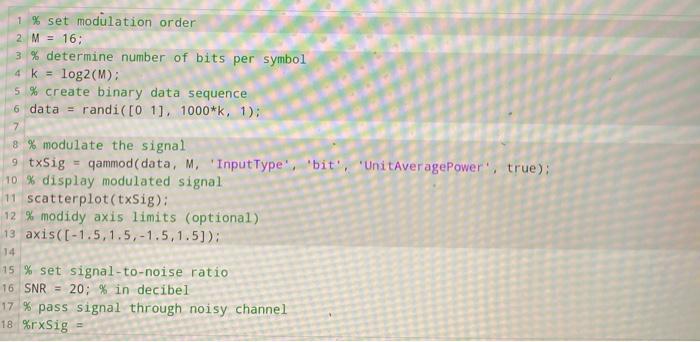
Running the script without any modifications will give you the constellation diagram (I/Q diagram) for 16-QAM. Your task is to simulate that the transmitted signal txSig passes a channel with additive white gaussian noise (so called AWGN). You can use the MATLAB function awgn to achieve that. The received signal should be called rxSig. While not neccessary in order to pass this problem, feel free to explore the behaviour of the system when you change the modulation (variable M) or change the signal-to-noise ration (variable SNR). For submitting please reset the variables M to be 16 and SNR to be 20. Running the script without any modifications will give you the constellation diagram (1/Q diagram) for 16-QAM. Your task is to simulate that the transmitted signal txSig passes a channel with additive white gaussian noise (so called AWGN). You can use the MATLAB function awgn to achieve that. The received signal should be called Sig. While not neccessary in order to pass this problem, feel free to explore the behaviour of the system when you change the modulation (variable M) or change the signal-to-noise ration (variable SNR). For submitting please reset the variables M to be 16 and SNR to be 20. Script C Reset MATLAB Documentation 1 % set modulation order 2 M = 16: 3% determine number of bits per symbol 4 K log2(M): 5 % create binary data sequence 6 data = randi( [0 11. 1000*k, 1); 7 8 % modulate the signal 9 txSig = qammod(data, M. "InputType''bit', 'UnitAveragePower', true); 10 % display modulated signal 11 scatterplot(txSig): 12 modidy axis limits optional 1 % set modulation order 2 M = 16; 3 % determine number of bits per symbol 4 k = log2(M): 5 % create binary data sequence 6 data = randi([01]. 1000*k, 1): 7 8 % modulate the signal 9 txSig - gammod(data, M. 'InputType', 'bit', 'UnitAveragePower", true): 10 % display modulated signal 11 scatterplot(txSig): 12 % modidy axis limits (optional) 13 axis([-1.5,1.5, -1.5,1.5)): 14 15 % set signal-to-noise ratio 16 SNR = 20; % in decibel 17% pass signal through noisy channel 18 %rxSig Running the script without any modifications will give you the constellation diagram (I/Q diagram) for 16-QAM. Your task is to simulate that the transmitted signal txSig passes a channel with additive white gaussian noise (so called AWGN). You can use the MATLAB function awgn to achieve that. The received signal should be called rxSig. While not neccessary in order to pass this problem, feel free to explore the behaviour of the system when you change the modulation (variable M) or change the signal-to-noise ration (variable SNR). For submitting please reset the variables M to be 16 and SNR to be 20. Running the script without any modifications will give you the constellation diagram (1/Q diagram) for 16-QAM. Your task is to simulate that the transmitted signal txSig passes a channel with additive white gaussian noise (so called AWGN). You can use the MATLAB function awgn to achieve that. The received signal should be called Sig. While not neccessary in order to pass this problem, feel free to explore the behaviour of the system when you change the modulation (variable M) or change the signal-to-noise ration (variable SNR). For submitting please reset the variables M to be 16 and SNR to be 20. Script C Reset MATLAB Documentation 1 % set modulation order 2 M = 16: 3% determine number of bits per symbol 4 K log2(M): 5 % create binary data sequence 6 data = randi( [0 11. 1000*k, 1); 7 8 % modulate the signal 9 txSig = qammod(data, M. "InputType''bit', 'UnitAveragePower', true); 10 % display modulated signal 11 scatterplot(txSig): 12 modidy axis limits optional 1 % set modulation order 2 M = 16; 3 % determine number of bits per symbol 4 k = log2(M): 5 % create binary data sequence 6 data = randi([01]. 1000*k, 1): 7 8 % modulate the signal 9 txSig - gammod(data, M. 'InputType', 'bit', 'UnitAveragePower", true): 10 % display modulated signal 11 scatterplot(txSig): 12 % modidy axis limits (optional) 13 axis([-1.5,1.5, -1.5,1.5)): 14 15 % set signal-to-noise ratio 16 SNR = 20; % in decibel 17% pass signal through noisy channel 18 %rxSig