MATLAB MATLAB

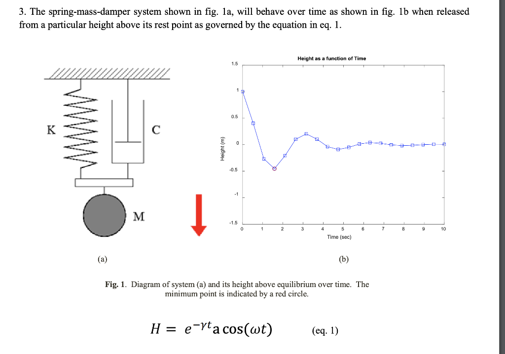
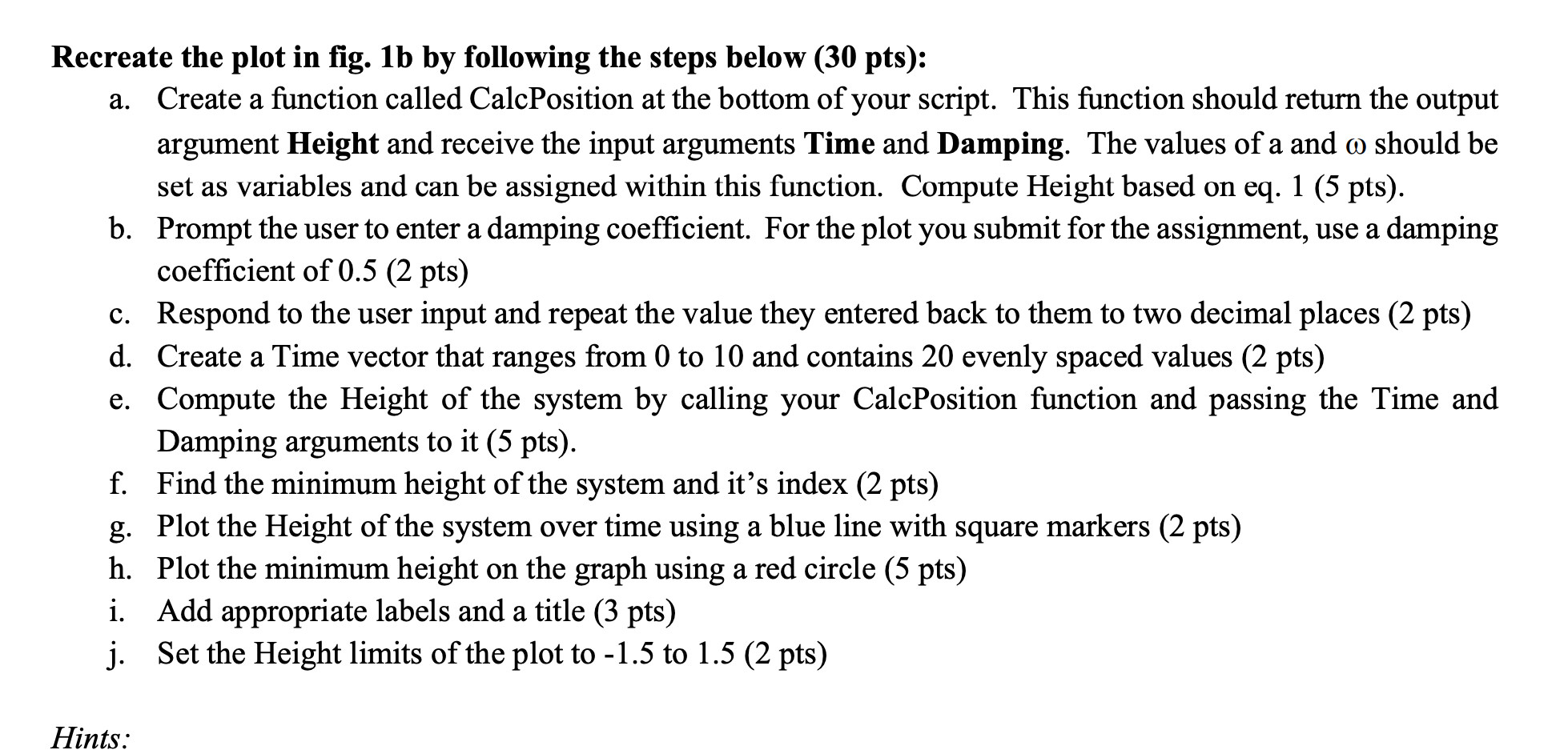
3. The spring-mass-damper system shown in fig. 1a, will behave over time as shown in fig. 1b when released from a particular height above its rest point as governed by the equation in eq. 1. Height as a function of Time Height (m) 0 1 2 3 4 6 7 8 9 10 5 Time (sec) (b) Fig. 1. Diagram of system (a) and its height above equilibrium over time. The minimum point is indicated by a red circle. H = e-rta cos(wt) (eq. 1) Recreate the plot in fig. 1b by following the steps below (30 pts): a. Create a function called CalcPosition at the bottom of your script. This function should return the output argument Height and receive the input arguments Time and Damping. The values of a and a should be set as variables and can be assigned within this function. Compute Height based on eq. 1 (5 pts). b. Prompt the user to enter a damping coefficient. For the plot you submit for the assignment, use a damping coefficient of 0.5 (2 pts) c. Respond to the user input and repeat the value they entered back to them to two decimal places (2 pts) d. Create a Time vector that ranges from 0 to 10 and contains 20 evenly spaced values (2 pts) e. Compute the Height of the system by calling your CalcPosition function and passing the Time and Damping arguments to it (5 pts). f. Find the minimum height of the system and it's index (2 pts) g. Plot the Height of the system over time using a blue line with square markers (2 pts) h. Plot the minimum height on the graph using a red circle (5 pts) i. Add appropriate labels and a title (3 pts) j. Set the Height limits of the plot to -1.5 to 1.5 (2 pts) Hints