(matlab only) (matlab only) (matlab only) (matlab only)

here is the question needed to be answered

here are some equations and graphs that will help

this should be al you need, pls help new code this I'm so confused

I WILL UPVOTE IF CODE WORKS

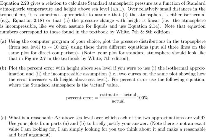
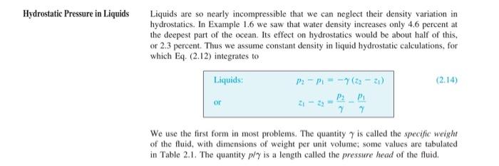
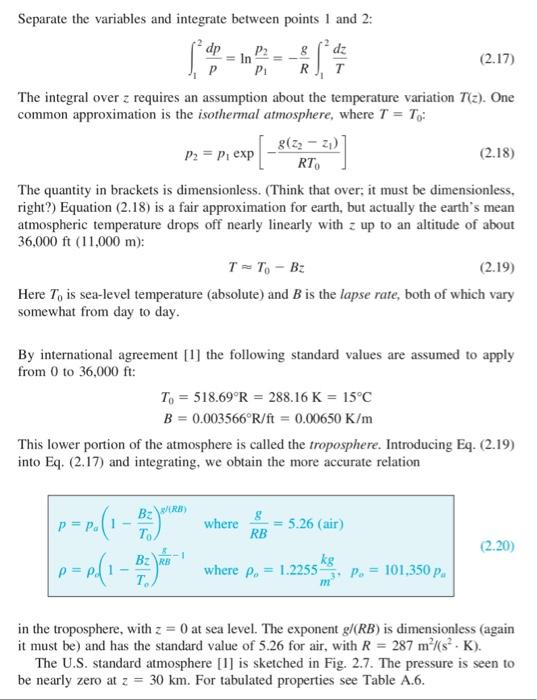
Equation 2.20 gives a relation to calculate Standard atmospheric pressure as a function of Standard atmospheric temperature and height above sea level (a.s.l.). Over relatively small distances in the troposphere, it is sometimes appropriate to assume that (i) the atmosphere is either isothermal (e.g., Equation 2.18) or that (ii) the pressure change with height is linear (i.e., the atmosphere is incompressible, like we often assume for liquids and use Equation 2.14). Note that equation numbers correspond to those found in the textbook by White, 7th & 8th editions. (a) Using the computer program of your choice, plot the pressure distributions in the troposphere (from sea level to ~ 10 km) using these three different equations (put all three lines on the same plot for direct comparison). (Note: your plot for standard atmosphere should look like that in Figure 2.7 in the textbook by White, 7th edition). (b) Plot the percent error with height above sea level if you were to use (i) the isothermal approx- imation and (ii) the incompressible assumption (i.e., two curves on the same plot showing how the error increases with height above sea level). For percent error use the following equation, where the Standard atmosphere is the 'actual' value. estimate - actual percent error -100% actual (C) What is a reasonable Az above sea level over which each of the two approximations are valid? Use your plots from parts (a) and (b) to briefly justify your answer. (Note there is not an exact value I am looking for, I am simply looking for you too think about it and make a reasonable and brief argument). Hydrostatic Pressure in Liquids Liquids are so nearly incompressible that we can neglect their density variation in hydrostatics. In Example 1.6 we saw that water density increases only 4.6 percent at the deepest part of the ocean. Its effect on hydrostatics would be about half of this, or 2.3 percent. Thus we assume constant density in liquid hydrostatic calculations, for which Eq. (2.12) integrates to Liquids P2-P--7(2-2) (2.14) or P2P 7 We use the first form in most problems. The quantity 7 is called the specific weight of the fluid, with dimensions of weight per unit volume; some values are tabulated in Table 2.1. The quantity ply is a length called the pressure head of the fluid. Separate the variables and integrate between points 1 and 2: dp P2 8 dz (2.17) P1 RIT The integral over z requires an assumption about the temperature variation T(z). One common approximation is the isothermal atmosphere, where T = To: 8(22 - 2 P2 = P, exp (2.18) RT The quantity in brackets is dimensionless. (Think that over, it must be dimensionless, right?) Equation (2.18) is a fair approximation for earth, but actually the earth's mean atmospheric temperature drops off nearly linearly with z up to an altitude of about 36,000 ft (11,000 m): TT. - B: (2.19) Here To is sea-level temperature (absolute) and B is the lapse rate, both of which vary somewhat from day to day. By international agreement [1] the following standard values are assumed to apply from 0 to 36,000 ft: T. = 518.69R = 288.16 K = 15C B = 0.003566R/ft = 0.00650 K/m This lower portion of the atmosphere is called the troposphere. Introducing Eq. (2.19) into Eq. (2.17) and integrating, we obtain the more accurate relation | p=p.(1-3 BR) where 5.26 (air) RB (2.20) B2 RB where p. = 1.2255 P. = 101,350 p. in the troposphere, with z = 0 at sea level. The exponent g/(RB) is dimensionless (again it must be) and has the standard value of 5.26 for air, with R = 287 m (s. K). The U.S. standard atmosphere [1] is sketched in Fig. 2.7. The pressure is seen to be nearly zero at 2 = 30 km. For tabulated properties see Table A.6