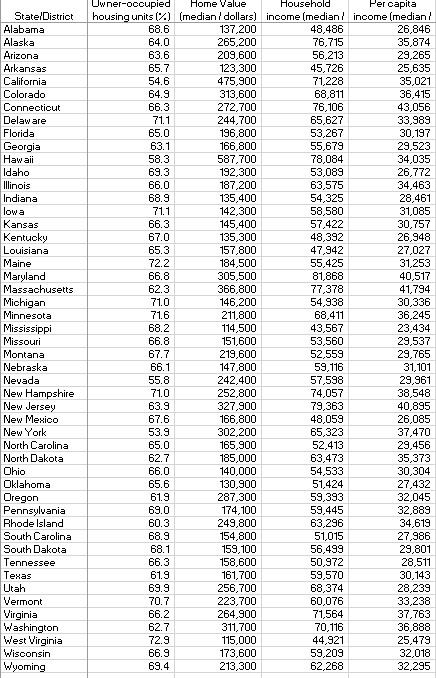
MBA 6350 Week 2 Case Study - Data Visualization and Descriptive Statistics (Case Study #2) Case Study #2 is intended to test your knowledge of how to summarize data into descriptive statistics and correlation analysis, as well as create histograms, boxplots, and scatterplots for the applicable variables. The data file contains estimated housing and income data for 2018 for each of the 50 US states per the American Community Survey. The data fields included are as follows: ? Owner-occupied housing units (%) - Pct Owner Occ ? Home Value (median / dollars) - Home Value ? Household income (median / dollars) - HH Inc ? Per capita income (median / dollars) - Per Cap Inc Prior to a more detailed analysis of the data, a company wants to get a good understanding of four of the variables: Home Value; HH Inc; Per Cap Inc; Pct Owner Occ (e.g. central tendency, variability, shape of the distribution, pattern of relationship between the variables). A company representative contracts with you to help with this process. To help the company get a better understanding of the data, you are asked to perform the following analysis steps: 1. Using Data>Data Analysis>Descriptive Statistics in Excel, calculate the mean, median, range and standard deviation of each variable and summarize the results in table. 2. Using Excel, create a frequency histogram for each variable to determine the shape of the distributions. Be sure to give each chart a title and label the axes clearly. 3. Using Excel, create boxplots for each variable. Be sure to give each chart a title and label the axes clearly. 4. Using Excel, create scatterplots of each variable with each other variable (hint: you should have 6 scatterplots). Be sure to give each chart a title and label the axes clearly. 5. Using Data>Data Analysis>Correlation in Excel, calculate the correlation coefficient each variable with each other variable. 6. In Word, write a summary report of the findings that includes the tables and charts from steps 1-5 and includes the following: MBA 6350 Week 2 Case Study - Data Visualization and Descriptive Statistics (Case Study #2) a. An introductory paragraph summarizes the purpose of the analysis. b. A section (1 or more paragraphs) describing what the tabular data from step 1 indicate about the central tendency, variability and distribution of each variable. For example, do the variables appear to be distributed in a symmetric or skewed pattern? c. A section (1 or more paragraphs) describing how the frequency histograms from step 2 and the boxplots from step 3 support and clarify the findings of the tabular data. Include in this section any evidence suggesting outliers in the data. d. A section (1 or more paragraphs) describing what the scatterplots from step 4 and correlations from step 5 indicate about the relationship between the various pairs of variables (e.g., are the variables related?, does the relationship appear to be linear or nonlinear?, is the direction of the relationship positive or negative?). e. A concluding paragraph summarizing the key findings of the analysis and making recommendations for the variable among HH Inc, Per Cap Inc and Pct Owner Occ that is most strongly correlated with Home Value. Submit a single Excel workbook showing all work for Steps 1-5 and a Word document of your summary report that addresses all parts of Step 6 and that also includes/interweaves all supporting tables and charts from Steps 1-5 (to tell a story with the data and through visualization means). Case Study #2 is due on Sunday by 11:59pm of Week 2.

Owner-occupied Home Value Household Per capita State/District housing units (X) (median / dollars) income (median ) income (median ) Alabama 68.6 137.200 48.486 26.846 Alaska 64.0 265,200 76,715 35.874 Arizona 63.6 203,600 56.213 29,265 Arkansas 65.7 123,300 45,726 25,635 California 54.6 475,300 71,228 35,021 Colorado 64.9 313,600 68,811 36.415 Connecticut 66.3 272.700 76,106 43,056 Delaware 71.1 244.700 65,627 33,983 Florida 65.0 136,800 53.267 30,197 Georgia 63.1 166,800 55,679 29,523 Hawaii 58.3 587.700 78.084 34,035 Idaho 69.3 192.300 53,089 26,772 Illinois 66.0 187.200 63,575 34,463 Indiana 68.9 135,400 54.325 28.461 low a 71.1 142.300 58.580 31,085 Kansas 66.3 145,400 57.422 30,757 Kentucky 67.0 135,300 48,392 26,948 Louisiana 65.3 157,800 47,942 27,027 Maine 72.2 184,500 55,425 31,253 Maryland 66.8 305,500 81,868 40,517 Massachusetts 62.3 366,800 77.378 41,794 Michigan 71.0 146,200 54,938 30,336 Minnesota 71.6 211,800 68,411 36,245 Mississippi 68.2 114.500 43,567 23,434 Missouri 66.8 151,600 53,560 29,537 Montana 67.7 219,600 52,559 29,765 Nebraska 66.1 147.800 59,116 31, 101 Nevada 55.8 242.400 57,598 29,361 New Hampshire 71.0 252,800 74,057 38,548 New Jersey 63.9 327.900 79,363 40,895 New Mexico 67.6 166.800 48,059 26,085 New York 53.9 302,200 65,323 37.470 North Carolina 65.0 165,300 52.413 29,456 North Dakota 62.7 185,000 63,473 35,373 Ohio 66.0 140,000 54,533 30,304 Oklahoma 65.6 130,300 51,424 27.432 Oregon 61.9 287.300 59,393 32,045 Pennsylvania 69.0 174,100 59.445 32,889 Rhode Island 60.3 249,800 63.236 34,619 South Carolina 68.9 154.800 51,015 27.986 South Dakota 68.1 159,100 56,499 29,801 Tennessee 66.3 158,600 50,972 28,511 Texas 61.9 161,700 59,570 30,143 Utah 69.9 256,700 68,374 28,239 Vermont 70.7 223,700 60,076 33,238 Virginia 66.2 264.300 71,564 37.763 Washington 62.7 311,700 70,116 36,888 West Virginia 72.9 115,000 44,921 25.479 Wisconsin 66.9 173,600 59.209 32,018 Wyoming 69.4 213,300 62.268 32.295