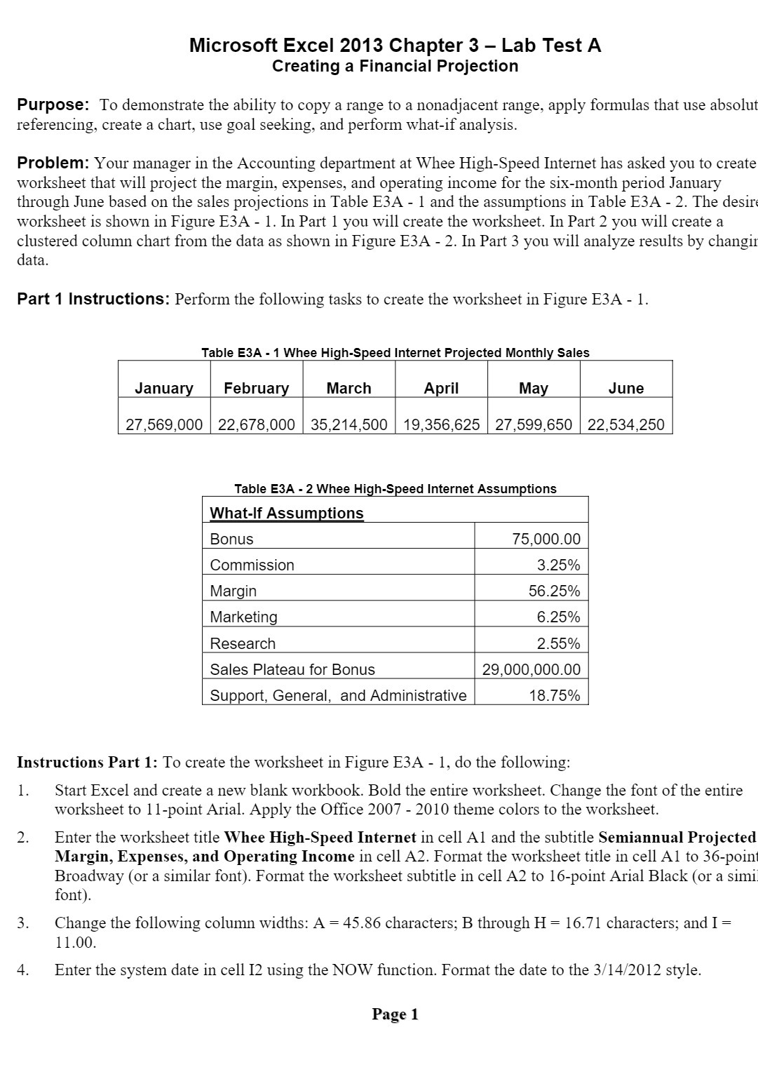
Microsoft Excel 2013 Chapter 3 Lab Test A Creating a Financial Projection Purpose: To demonstrate the ability to copy a range to a nonadj acent range, apply formulas that use absolut referencing, create a chart, use goal seeking, and perform what-if analysis. Problem: Your manager in the Accounting department at Whee Hi gh-Speed Internet has asked you to create worksheet that will project the margin, expenses, and operating income for the six-month period January through June based on the sales projections in Table E3A - l and the assumptions in Table E3A - 2. The desirt worksheet is shown in Figure E3A - 1. In Part 1 you will create the worksheet. In Part 2 you will create a clustered column chart from the data as shown in Figure E3A - 2. In Part 3 you will analyze results by changir data. Part 1 Instructions: Perform the following tasks to create the worksheet in Figure E3A - 1. Table E3A - 1 Whee High-Speed Internet Projected Monthly Sales Janua Februa March A ril Ma June 27,569,000 22,678,000 35,214,500 19,356,625 27,599,650 22,534,250 Table E3A - 2 Whee Hi . What-If Assumptions Bonus 75,000.00 Commission 3.25% Margin 56.25% Marketing 6.25% Research 2.55% Sales Plateau for Bonus 29,000,00000 Support, General, and Administrative 18.75% Instructions Part 1: To create the worksheet in Figure E3A - 1, do the following: 1. Start Excel and create a new blank workbook. Bold the entire worksheet. Change the font of the entire worksheet to 11-point Arial. Apply the Office 2007 - 2010 theme colors to the worksheet. Enter the worksheet title Whee High-Speed Internet in cell A1 and the subtitle Semiannual Projected Margin, Expenses, and Operating Income in cell A2. Format the worksheet title in cell Al to 36-point Broadway (or a similar font). Format the worksheet subtitle in cell A2 to 16-point Arial Black (or a simii font). Change the following column widths: A = 45.86 characters; B through H = 16.71 characters; and I = 1 1.00. Enter the system date in cell 12 using the NOW function. Format the date to the 31' 1412012 style. Page 1