Modify the following Code to exactly look like the plot given below and correct if some mistakes :

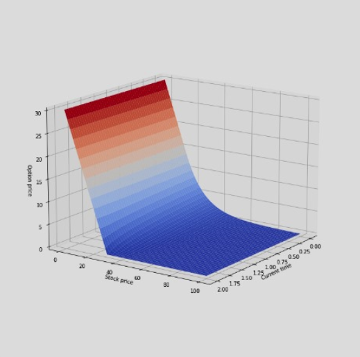
values :

#values - S = 50 , K = 50.0, r = 0.1, q =0, sigma = 0.4, T = 5/12, M= 20, N= 10 #values - S0 = 100 K = 30 r = 0.05 sigma = 0.2 T = 2 Sinf = 2 * K M = 100 N = 100

Current output with sample values :

pde.py:

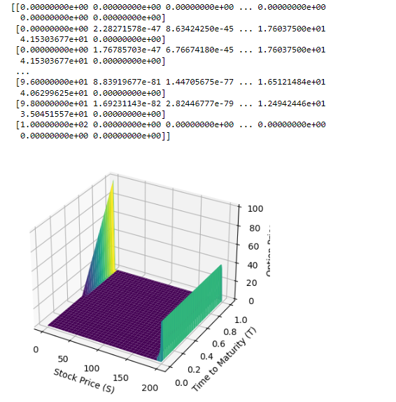
#!/usr/bin/env python # coding: utf-8 # In[1]: import numpy as np from scipy.optimize import fsolve from scipy.interpolate import interp2d from typing import Callable #Implementing the use of a class to solve the BSM PDE using the implicit finite difference scheme. class BSMPDESolver: def __init__(self, spot_price, strike_price, maturity, volatility, interest_rate, dividend_yield, payoff_function: Callable): self.S = spot_price self.K = strike_price self.T = maturity self.sigma = volatility self.r = interest_rate self.q = dividend_yield self.payoff_function = payoff_function def solve_pde(self, option_type='European', grid_size=(100, 100)): M, N = grid_size dt = self.T / M dS = (2 * self.S) / N # Initialize grid S_values = np.linspace(0, 2 * self.S, N + 1) t_values = np.linspace(0, self.T, M + 1) grid = np.zeros((M + 1, N + 1)) # Set boundary conditions grid[:, 0] = self.payoff_function(S_values) grid[:, -1] = 0 if option_type == 'European' else self.K - S_values[-1] # Solve the implicit finite difference scheme for i in range(M - 1, 0, -1): A = self._build_coefficient_matrix(grid[i + 1, 1:-1], dS, dt) B = self._build_rhs_vector(grid[i + 1, 1:-1], dS, dt, S_values[1:-1], t_values[i]) grid[i, 1:-1] = fsolve(lambda x: np.dot(A, x) - B, grid[i, 1:-1]) return S_values, t_values, grid def _build_coefficient_matrix(self, u_next, dS, dt): sigma2 = self.sigma**2 r = self.r q = self.q alpha = 0.5 * dt * (sigma2 * np.arange(1, len(u_next) + 1)**2 - (r - q) * np.arange(1, len(u_next) + 1)) beta = 1 + dt * (sigma2 * np.arange(1, len(u_next) + 1)**2 + r) gamma = -0.5 * dt * (sigma2 * np.arange(1, len(u_next) + 1)**2 + (r - q) * np.arange(1, len(u_next) + 1)) A = np.diag(alpha[:-1], -1) + np.diag(beta) + np.diag(gamma[:-1], 1) return A def _build_rhs_vector(self, u_next, dS, dt, S_values, t): sigma2 = self.sigma**2 r = self.r q = self.q b = u_next.copy() b[0] -= 0.5 * dt * (sigma2 * 1**2 - (r - q) * 1) * (self.payoff_function(S_values[0]) - self.payoff_function(S_values[0] - dS)) b[-1] -= 0.5 * dt * (sigma2 * len(u_next)**2 + (r - q) * len(u_next)) * (self.K - S_values[-1]) return b # Sample question : if __name__ == "__main__": def payoff_function(S): return np.maximum(0, S - 100) # Example payoff function (call option) bsm_solver = BSMPDESolver(spot_price= 50, strike_price=100, maturity=1, volatility=0.2, interest_rate=0.05, dividend_yield=0.02, payoff_function=payoff_function) S_values, t_values, option_prices = bsm_solver.solve_pde(option_type='European') # Print or visualize the results as needed print(option_prices) # In[ ]:

pde_plots.ipnyb :

import matplotlib.pyplot as plt from mpl_toolkits.mplot3d import Axes3D import pde import numpy as np if __name__ == "__main__": def payoff_function(S): return np.maximum(0, S - 100) # Example payoff function (call option) bsm_solver = pde.BSMPDESolver(spot_price=100, strike_price=100, maturity=1, volatility=0.2, interest_rate=0.1, dividend_yield=0.02, payoff_function=payoff_function) S_values, t_values, option_prices = bsm_solver.solve_pde(option_type='European') # Print or visualize the results as needed print(option_prices) # Assuming option_prices is the result from your PDE solver fig = plt.figure() ax = fig.add_subplot(111, projection='3d') X, Y = np.meshgrid(S_values, t_values) ax.plot_surface(X, Y, option_prices, cmap='viridis') ax.set_xlabel('Stock Price (S)') ax.set_ylabel('Time to Maturity (T)') ax.set_zlabel('Option Price') plt.show()

1 [[0.00000000e+000.00000000e+000.00000000e+000.00000000e+00 0.00000000e+000.00000000e+00] 4.15303677e+010.00000000e+00] 4.15303677e+010.00000000e+00] ... [9.60000000e+01 8.83919677e-81 1.44705675e-77 ... 1.65121484e+01 4.06299625e+010.00000000e+00] [9.80000000e+011.69231143e822.82446777e79.1.24942446e+01 3.50451557e+010.00000000e+00] 0.00000000e+000.00000000e+00] ]