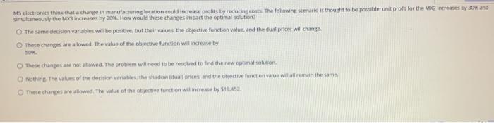
Question: MS electronics think that change in manufacturing location could increase profits by reducing the following scenario is thought to be possible unit profit for the

MS electronics think that change in manufacturing
MS electronics think that change in manufacturing location could increase profits by reducing the following scenario is thought to be possible unit profit for the MX2 increases by 30% and simultaneously the increases by 2011. How would these changes mpact the optimal solution? The same decision variables will be positive, but their values the bjective function value and the dual prices will change These changes are allowed. The value of the objective function will create by These changes are not allowed. The problem will need to be resolved to find the new optimal solution Nothing the values of the decision variables the shadows and the otjective function value will remain the same These changes are allowed. The value of the objective function will increase by 5145 MS electronics supply highly complex components for military communications systems. Four products, named the MX range, share the labor hours available for each of the four production processes: wiring, drilling, assembly and finishing. For each product and each process, the hours of labor required for each unit of production and the total hours available per month are shown in the table below. The table also shows the profit earned per unit for each product and the minimum monthly demand for that product. Product Hours of labour per production unit Profit Minimum per unit (type of component) Wiring Drilling Assembly Finishing Demand ($) Time Time Time Time (no. of units) MX1 0.5 0.6 0.2 0.5 20 15000 MX2 1.5 1.0 3.5 0.9 30 500 MX3 3.0 1.5 1.0 0.5 35 1800 MX4 1.0 2.5 2.0 0.6 25 900 Labor available 16000 18000 12000 10000 (hours per month) Variable Cells Cell Name $B$2 MX1 $C$2 MX2 $D$2 MX3 $E$2 MX4 Original Value 0 0 0 0 Final Value 15884 500 2136 900 Integer Contin Contin Contin Contin Constraints Cell $F$10 $F$11 $F$12 $F$5 $F$6 $F$7 $F$8 $F$9 Name Dem (MX2) Dem (MX3) Dem (MX4) Wiring Drilling Assembly Finishing Dem (MX1) Cell Value 500 2136 900 16000 15484.4 8862.8 10000 15884 Formula $F$10>$H$10 $F$11>$H$11 $F$12>=$H$12 $F$5=$H$9 Status Binding Not Binding Binding Binding Not Binding Not Binding Binding Not Binding Slack 0 336 0 0 2515.6 3137.2 0 884 Variable Cells Cell $B$2 $C$2 $D$2 SE$2 Constraints Name MX1 MX2 MX3 MX4 Final Value 15884 500 2136 900 Reduced Cost 0 0 0 0 Objective Coefficient 20 30 35 25 Allowable Increase 15 9.6 85 Allowable Decrease 1.35 1E+30 8.75 1E+30 1.4 Cell $F$10 $F$11 $F$12 SFS5 SF$6 SF$7 SF$8 SF99 Name Dem (MX2) Dem (MX3) Dem (MX4) Wiring Drilling Assembly Finishing Dem (MX1) Final Value 500 2136 900 16000 15484 8863 10000 15884 Shadow Price -9.6 0 -1.4 6 Constraint R.H. Side 500 1800 900 16000 18000 12000 10000 Allowable Increase 566.7 336 850 2210 1E+30 1E+30 840 884 Allowable Decrease 500 1E+30 900 840 2515.6 31372 368.3 1E30 0 O 34 15000

Step by Step Solution

There are 3 Steps involved in it

1 Expert Approved Answer
Step: 1 Unlock blur-text-image
Question Has Been Solved by an Expert!

Get step-by-step solutions from verified subject matter experts

Step: 2 Unlock
Step: 3 Unlock

Students Have Also Explored These Related General Management Questions!