Need help with partB AND C

Lab 2: Numerical Methods

This Maple lab is closely based on earlier versions prepared by Professors R. Falk and R. Bumby of the Rutgers Mathematics department.

Introduction. In this lab, we shall use Maples ability to approximate the solution of differential equations by numerical methods and superimpose these solutions on the direction fields that we studied in Lab 1. This allows us to extend our understanding of the solutions of differential equations to equations for which a closed form solution is not available.

Please obtain the seed file from the web page and save it in your directory on eden, then prepare the Maple lab according to the instructions and hints in the introduction to Lab 0. Turn in only the printout of your Maple worksheet, after removing any extraneous material and any errors you have made.

Setup. As usual, the seed file begins with commands which load the required Maple packages: with(plots): and with(DEtools): .

Equation 1.

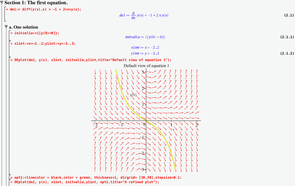
a. One Solution. The sequence of commands to begin working with Equation 1 have already been entered into the seed file. Execute them to see how Maple can be used to plot the direction field along with the particular solution satisfying this differential equation and the initial condition y(0) = 0. The quantities x1int and y1int are introduced to have standard names for the ranges of the variables in all graphs in this problem. For the other exercises, corresponding commands can be constructed by copying lines to different places in a worksheet and doing some minor editing.

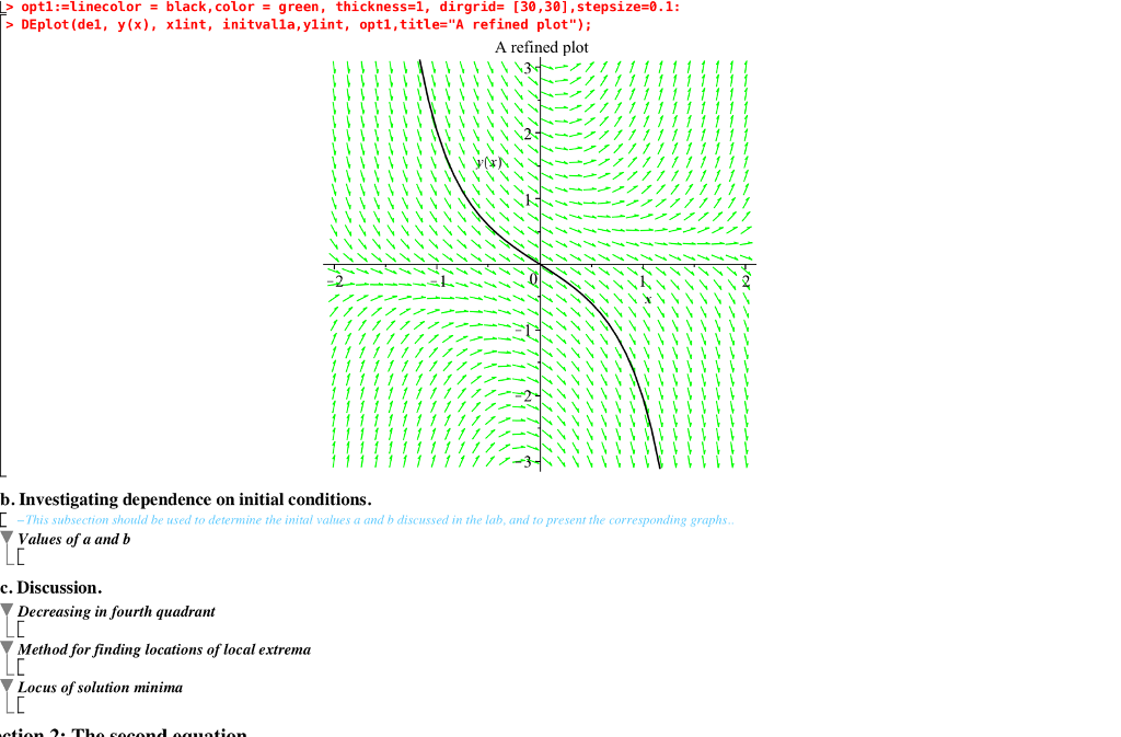
 de1:= diff(y(x),x) = -1 + 2*x*y(x) initval1a:={[y(0)=0]}; x1int:=x=-2..2;y1int:=y=-3..3; DEplot(de1, y(x), x1int, initval1a,y1int,title="Default view of equation 1"); 

The DEplot command has many options which you can read about in the Maple help pages. In particular, it is possible to specify the color and width of the solution curve by using linecolor and thickness, the color of the direction field by using color, to make the gridwork of lines in the direction field finer (or coarser) by using the dirfield option, and to get a finer resolution in computing the solution with the stepsize option. For example, try:

 opt1:=linecolor = black,color = green, thickness=1, dirfield= [30,30], stepsize=0.1; 

 DEplot(de1, y(x), x1int, initval1a, y1int, opt1,title= "A refined plot"); 

b. Dependence on initial condition. By varying the initial conditions, it is possible to approximate special solutions. For example, one type of solution of this equation, e.g. the one with with y(0) = 0, is everywhere decreasing, whereas another type, e.g. the one with y(0) = 2 reaches a minimum value and then becomes rapidly increasing as x +. By plotting solutions with other values of y(0) between 0 and 2, you can identify more precisely where this change of behavior occurs. To investigate this behavior, copy the first three command lines under part a to part (b), change the range of x to go from -1 to 3, and experiment by graphing the solution with different initial values y(0). Find two initial values a and b, satisfying 0

(c) Qualitative properties. Many qualitative properties of solutions of a differential equation can be determined from the equation itself. These qualitative properties serve as a check against obvious

opt1 line color black, color green thickness l, dirgrid- 30,301, stepsize30.1 DEplot (del, y (x), xlint initvalla, ylint optl title-"A refined plot") A refined plot 1 1 1 1 1 1 1 1 1 1 1 1 1 1 1 1 1 1 1 1 1 NNNYN NNNNNN 1 1 1 1 1 11 1 1 1 1 1 1 1 1 1 1 1 1 1 1 1 1 1 1 1 1 1 1 1 1 1 1 1 1 1 1 1 1 1 1 1 f 1 1 1 1 1 1 1 11 1 1 1 1 1 1 b. Investigating dependence on initial conditions. This subsection should be used to determine the inital values a and b discussed in the lab, and to present the corresponding graphs values of a and b c. Discussion Decreasing in fourth quadrant Method for finding locations of local extrema Locus of solution minima opt1 line color black, color green thickness l, dirgrid- 30,301, stepsize30.1 DEplot (del, y (x), xlint initvalla, ylint optl title-"A refined plot") A refined plot 1 1 1 1 1 1 1 1 1 1 1 1 1 1 1 1 1 1 1 1 1 NNNYN NNNNNN 1 1 1 1 1 11 1 1 1 1 1 1 1 1 1 1 1 1 1 1 1 1 1 1 1 1 1 1 1 1 1 1 1 1 1 1 1 1 1 1 1 f 1 1 1 1 1 1 1 11 1 1 1 1 1 1 b. Investigating dependence on initial conditions. This subsection should be used to determine the inital values a and b discussed in the lab, and to present the corresponding graphs values of a and b c. Discussion Decreasing in fourth quadrant Method for finding locations of local extrema Locus of solution minima