Need solutions for solving 4.4 and 4.8 using python. Questions are attached as a screenshot.

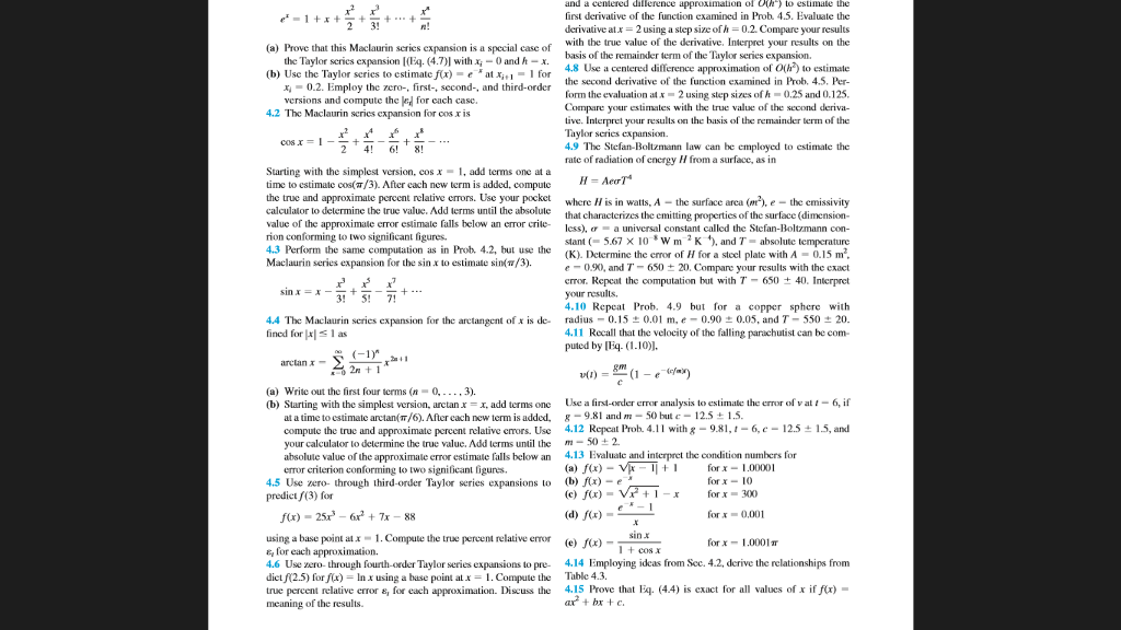
and a centered dallerence approximation o O) to estimate the first derivative of the function examined in Prob. 4.5. Evaluate the derivative at x 2 using a step size ofh-0.2 Compare your results with the true value of the derivative. Interpret your results on the basis of the remainder term of the Taylor series expansion. 2 3! rn! (a) Prove that this Maclaurin serics expansion is a special case of W the T r scrics expansion I(Eq. (4.7) wth-O and /t-x.4.8 Use a centered difference a approximation of O(h to estimate (b) Usc the Taylor scries to estimatc fx)-e at -1 for the second derivative of the function examined in Prob, 4.5, Per- form the evaluation at x 2 using step sizes of h-0.25 and 0.125. Compare your estimales with the true value of the second deriva- tive. Interpret your results on the basis of the remainder term of the Taylor serics expansion. 4.9 The Stefan-Boltzmann law can be employed to cstimatc the rate of radiation of energy H from a surface, as in x,-02. Employ the zero-, first-, second-, and third-order versions and compute the for each case. for cos x is cos x = 1 Starting with the simplest version, cosx 1, add terms one at a time to estimate cos(/3). After each new term is added, compute the true and approximate percent relative crrors. Use your pockct where H is in watts, A -the surface arca (m2, e themissivity calculalor lo delermine the true value. Add lerms until the absolule value of the approximale error estimale falls below an error crile- rion conforming to two signilicant figures. 4.3 Perform the same computation as in Prob. 4.2, but use the K). Dcterminc the error of H for a stcel plate with A 0.15 m2 Maclaurin series expansion for the sin x 10 estimale sin(/3). H=AerT4 that characterizes the emitting properties of the surface (dimcnsion- less), a universal constant called the Stefan-Boltzmann con- stant 5.67 X 10W m K , and T- absolute temperature e-0.90. and T-650 20, Compare your results with the exact error. Repeat the computation but with T-650 40. Internet your results 4.10 Repeat Prob. 4.9 but for a copper sphere with radius 4.11 Recall that the velocity of the falling parachutist can be com puted by [Eq(10) sinx=x--+ + 4.4 The Maclaurin serie sexpansion for the arctangent of x is de- fined for 1 as 0.15 0.01 m. e-0.900.05, and T-55020. n11 arctan X 2n 1 grm (a) write out the first four terms (n-0,- 3). (b) Starting with the samplest version, arctan x 6, if Use a find order error analysis to estimate the error o g 9.81 and m-SO but c-125tLs. 4.12 Repeat Prob 4.11 with g 981, 6, e 125-i5, and add terms one ra , at a time to estimate arctan(m/6). After cach new term is added, compute the true and approximate percent relative crors. Use your calculator to determine the true value. Add lerms until the absolute value of the approximale error estimale falls below an error criterion conforming to two significant ligunes m-50 2. (a) f(x)-vp (c) f(x)-V+-xorx300 4.13 Evaluate and interpret the condition numbers for for x 1.00001 for x-0 +1 4.5 Use zero- through third-order Taylor series expansions to (b)-e predict (3) for x)-25x-67x 88 or x0,001 sin X efrom See. 4.2 using a base point a1. Compute the true percent relative error f, for each approximation 4.6 Use zero through fourth-order Taylor series expansions to pre 4.14 Employing ideas from Sce. 4.2, derive the relationships from dictf2.5) forf(x)-In x using a base point al x = 1. Compute the Table 4.3. true percent relative error &, for each approximation. Discuss the 4.S Pe that E(4.4) is exact for all values of x if fx) meaning of the results. for x-1.000! and a centered dallerence approximation o O) to estimate the first derivative of the function examined in Prob. 4.5. Evaluate the derivative at x 2 using a step size ofh-0.2 Compare your results with the true value of the derivative. Interpret your results on the basis of the remainder term of the Taylor series expansion. 2 3! rn! (a) Prove that this Maclaurin serics expansion is a special case of W the T r scrics expansion I(Eq. (4.7) wth-O and /t-x.4.8 Use a centered difference a approximation of O(h to estimate (b) Usc the Taylor scries to estimatc fx)-e at -1 for the second derivative of the function examined in Prob, 4.5, Per- form the evaluation at x 2 using step sizes of h-0.25 and 0.125. Compare your estimales with the true value of the second deriva- tive. Interpret your results on the basis of the remainder term of the Taylor serics expansion. 4.9 The Stefan-Boltzmann law can be employed to cstimatc the rate of radiation of energy H from a surface, as in x,-02. Employ the zero-, first-, second-, and third-order versions and compute the for each case. for cos x is cos x = 1 Starting with the simplest version, cosx 1, add terms one at a time to estimate cos(/3). After each new term is added, compute the true and approximate percent relative crrors. Use your pockct where H is in watts, A -the surface arca (m2, e themissivity calculalor lo delermine the true value. Add lerms until the absolule value of the approximale error estimale falls below an error crile- rion conforming to two signilicant figures. 4.3 Perform the same computation as in Prob. 4.2, but use the K). Dcterminc the error of H for a stcel plate with A 0.15 m2 Maclaurin series expansion for the sin x 10 estimale sin(/3). H=AerT4 that characterizes the emitting properties of the surface (dimcnsion- less), a universal constant called the Stefan-Boltzmann con- stant 5.67 X 10W m K , and T- absolute temperature e-0.90. and T-650 20, Compare your results with the exact error. Repeat the computation but with T-650 40. Internet your results 4.10 Repeat Prob. 4.9 but for a copper sphere with radius 4.11 Recall that the velocity of the falling parachutist can be com puted by [Eq(10) sinx=x--+ + 4.4 The Maclaurin serie sexpansion for the arctangent of x is de- fined for 1 as 0.15 0.01 m. e-0.900.05, and T-55020. n11 arctan X 2n 1 grm (a) write out the first four terms (n-0,- 3). (b) Starting with the samplest version, arctan x 6, if Use a find order error analysis to estimate the error o g 9.81 and m-SO but c-125tLs. 4.12 Repeat Prob 4.11 with g 981, 6, e 125-i5, and add terms one ra , at a time to estimate arctan(m/6). After cach new term is added, compute the true and approximate percent relative crors. Use your calculator to determine the true value. Add lerms until the absolute value of the approximale error estimale falls below an error criterion conforming to two significant ligunes m-50 2. (a) f(x)-vp (c) f(x)-V+-xorx300 4.13 Evaluate and interpret the condition numbers for for x 1.00001 for x-0 +1 4.5 Use zero- through third-order Taylor series expansions to (b)-e predict (3) for x)-25x-67x 88 or x0,001 sin X efrom See. 4.2 using a base point a1. Compute the true percent relative error f, for each approximation 4.6 Use zero through fourth-order Taylor series expansions to pre 4.14 Employing ideas from Sce. 4.2, derive the relationships from dictf2.5) forf(x)-In x using a base point al x = 1. Compute the Table 4.3. true percent relative error &, for each approximation. Discuss the 4.S Pe that E(4.4) is exact for all values of x if fx) meaning of the results. for x-1.000