need to code a plot on matlab

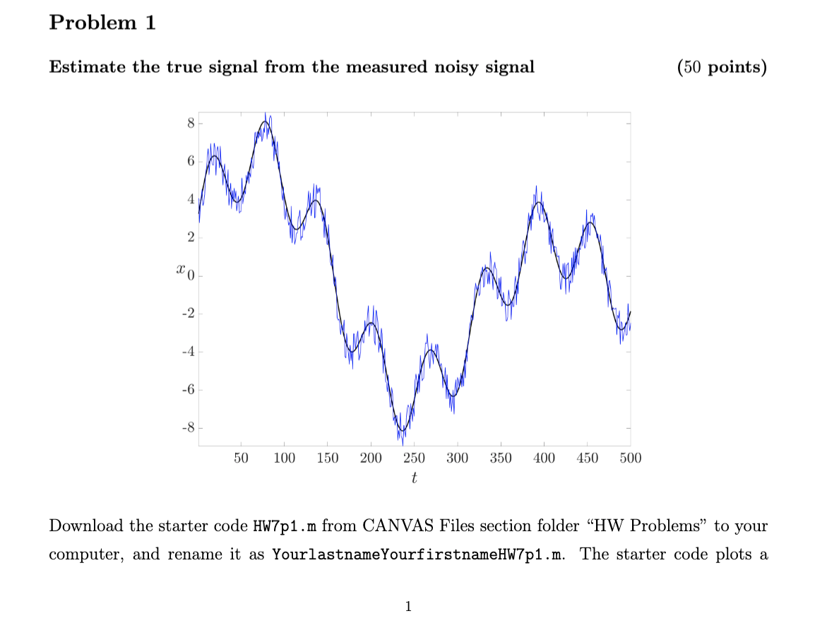
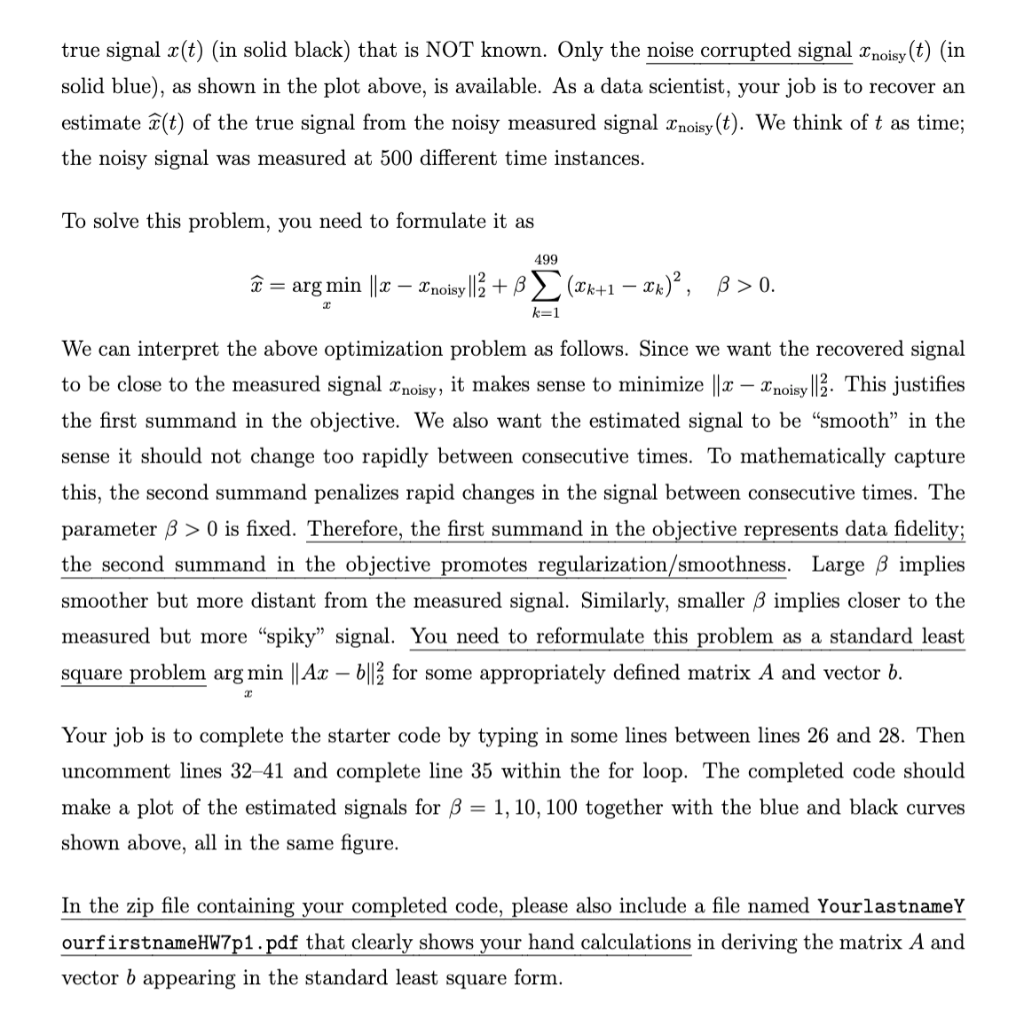
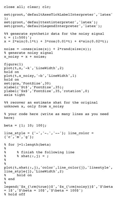
Problem 1 Estimate the true signal from the measured noisy signal (50 points) 8 6 2 20 -2 -4 -6 -8 50 100 150 200 250 300 350 400 450 500 t Download the starter code Hw7p1.m from CANVAS Files section folder "HW Problems to your computer, and rename it as YourlastnameyourfirstnameHW7p1.m. The starter code plots a 1 true signal x(t) (in solid black) that is NOT known. Only the noise corrupted signal 2noisy(t) (in solid blue), as shown in the plot above, is available. As a data scientist, your job is to recover an estimate (t) of the true signal from the noisy measured signal Inoisy(t). We think of t as time; the noisy signal was measured at 500 different time instances. To solve this problem, you need to formulate it as 499 a = arg min || 2 Inoisy |13 + B (2x+1 xx)?, B >0. k=1 We can interpret the above optimization problem as follows. Since we want the recovered signal to be close to the measured signal 2noisy, it makes sense to minimize || 2 Znoisy ||2. This justifies the first summand in the objective. We also want the estimated signal to be smooth in the sense it should not change too rapidly between consecutive times. To mathematically capture this, the second summand penalizes rapid changes in the signal between consecutive times. The parameter > 0 is fixed. Therefore, the first summand in the objective represents data fidelity; the second summand in the objective promotes regularization/smoothness. Large implies smoother but more distant from the measured signal. Similarly, smaller 8 implies closer to the measured but more spiky" signal. You need to reformulate this problem as a standard least square problem arg min || Ax b||for some appropriately defined matrix A and vector b. Your job is to complete the starter code by typing in some lines between lines 26 and 28. Then uncomment lines 3241 and complete line 35 within the for loop. The completed code should make a plot of the estimated signals for B = 1, 10, 100 together with the blue and black curves shown above, all in the same figure. In the zip file containing your completed code, please also include a file named YourlastnameY ourfirstnameHW7p1.pdf that clearly shows your hand calculations in deriving the matrix A and vector b appearing in the standard least square form. close all; clear; clc; set (groot, 'defaultAxesTickLabelInterpreter', 'latex ); set (groot, 'defaulttextinterpreter', 'latex'); set (groot, 'defaultLegendInterpreter', 'latex'); $$ generate synthetic data for the noisy signal t = (1:500); x = 2*sin(0.1*t) + 3* cos(0.01*t) + 4+sin(0.02*t); noise = -ones (size(x)) + 2*rand(size(x)); $ generate noisy signal X_noisy - x + noise; figure(1) plot(t,x,'-', LineWidth', 2) hold on plot(t,x_noisy,'-b', 'LineWidth',1) hold on set (gca, 'FontSize', 30) xlabel('$t$', 'FontSize',35); ylabel('$X$', 'FontSize 35, rotation',0) axis tight $$ recover an estimate xhat for the original unknown x, only from x_noisy your code here (write as many lines as you need here) beta = [1; 10; 100); line_style = {'-,'-,'--'}; line_color ['c','m','g'}; & for j=1:length(beta) & finish the following line xhat(:,1); % 8 % plot(t, xhat (:,1), 'color'line_color{j}, 'linestyle', line_style{j}, 'LineWidth', 2) hold on 8 % end legend('$x_{ m{true}}$', '$x_{ m{noisy}}$', '$\beta = i', $\beta = 10$', 'S\beta = 100$) % hold off Problem 1 Estimate the true signal from the measured noisy signal (50 points) 8 6 2 20 -2 -4 -6 -8 50 100 150 200 250 300 350 400 450 500 t Download the starter code Hw7p1.m from CANVAS Files section folder "HW Problems to your computer, and rename it as YourlastnameyourfirstnameHW7p1.m. The starter code plots a 1 true signal x(t) (in solid black) that is NOT known. Only the noise corrupted signal 2noisy(t) (in solid blue), as shown in the plot above, is available. As a data scientist, your job is to recover an estimate (t) of the true signal from the noisy measured signal Inoisy(t). We think of t as time; the noisy signal was measured at 500 different time instances. To solve this problem, you need to formulate it as 499 a = arg min || 2 Inoisy |13 + B (2x+1 xx)?, B >0. k=1 We can interpret the above optimization problem as follows. Since we want the recovered signal to be close to the measured signal 2noisy, it makes sense to minimize || 2 Znoisy ||2. This justifies the first summand in the objective. We also want the estimated signal to be smooth in the sense it should not change too rapidly between consecutive times. To mathematically capture this, the second summand penalizes rapid changes in the signal between consecutive times. The parameter > 0 is fixed. Therefore, the first summand in the objective represents data fidelity; the second summand in the objective promotes regularization/smoothness. Large implies smoother but more distant from the measured signal. Similarly, smaller 8 implies closer to the measured but more spiky" signal. You need to reformulate this problem as a standard least square problem arg min || Ax b||for some appropriately defined matrix A and vector b. Your job is to complete the starter code by typing in some lines between lines 26 and 28. Then uncomment lines 3241 and complete line 35 within the for loop. The completed code should make a plot of the estimated signals for B = 1, 10, 100 together with the blue and black curves shown above, all in the same figure. In the zip file containing your completed code, please also include a file named YourlastnameY ourfirstnameHW7p1.pdf that clearly shows your hand calculations in deriving the matrix A and vector b appearing in the standard least square form. close all; clear; clc; set (groot, 'defaultAxesTickLabelInterpreter', 'latex ); set (groot, 'defaulttextinterpreter', 'latex'); set (groot, 'defaultLegendInterpreter', 'latex'); $$ generate synthetic data for the noisy signal t = (1:500); x = 2*sin(0.1*t) + 3* cos(0.01*t) + 4+sin(0.02*t); noise = -ones (size(x)) + 2*rand(size(x)); $ generate noisy signal X_noisy - x + noise; figure(1) plot(t,x,'-', LineWidth', 2) hold on plot(t,x_noisy,'-b', 'LineWidth',1) hold on set (gca, 'FontSize', 30) xlabel('$t$', 'FontSize',35); ylabel('$X$', 'FontSize 35, rotation',0) axis tight $$ recover an estimate xhat for the original unknown x, only from x_noisy your code here (write as many lines as you need here) beta = [1; 10; 100); line_style = {'-,'-,'--'}; line_color ['c','m','g'}; & for j=1:length(beta) & finish the following line xhat(:,1); % 8 % plot(t, xhat (:,1), 'color'line_color{j}, 'linestyle', line_style{j}, 'LineWidth', 2) hold on 8 % end legend('$x_{ m{true}}$', '$x_{ m{noisy}}$', '$\beta = i', $\beta = 10$', 'S\beta = 100$) % hold off