Any help with this MATLAB problem would be helpful.

STARTER CODE:

close all; clear; clc;

set(groot,'defaultAxesTickLabelInterpreter','latex');

set(groot,'defaulttextinterpreter','latex');

set(groot,'defaultLegendInterpreter','latex');

%% generate synthetic data for the noisy signal

t = (1:500)';

x = 2*sin(0.1*t) + 3*cos(0.01*t) + 4*sin(0.02*t);

noise = -ones(size(x)) + 2*rand(size(x));

% generate noisy signal

x_noisy = x + noise;

figure(1)

plot(t,x,'-k','LineWidth',2)

hold on

plot(t,x_noisy,'-b','LineWidth',1)

hold on

set(gca,'FontSize',30)

xlabel('$t$','FontSize',35); ylabel('$x$','FontSize',35,'rotation',0)

axis tight

%% recover an estimate xhat for the original unknown x, only from x_noisy

% your code here (write as many lines as you need here)

beta = [1; 10; 100];

line_style = {'-','-.','--'}; line_color = {'c','m','g'};

% for j=1:length(beta)

%

% % finish the following line

% % xhat(:,j) = ;

%

% plot(t,xhat(:,j),'color',line_color{j},'linestyle',line_style{j},'LineWidth',2)

% hold on

% end

% legend('$x_{ m{true}}$','$x_{ m{noisy}}$','$\beta = 1$','$\beta = 10$','$\beta = 100$')

% hold off

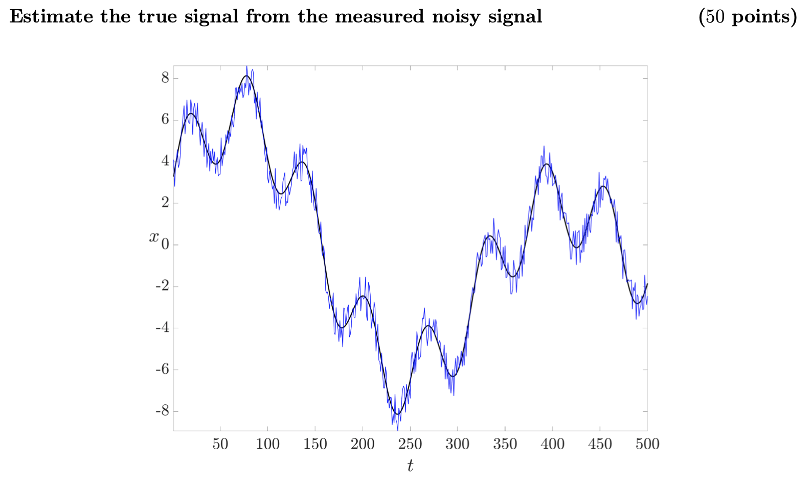
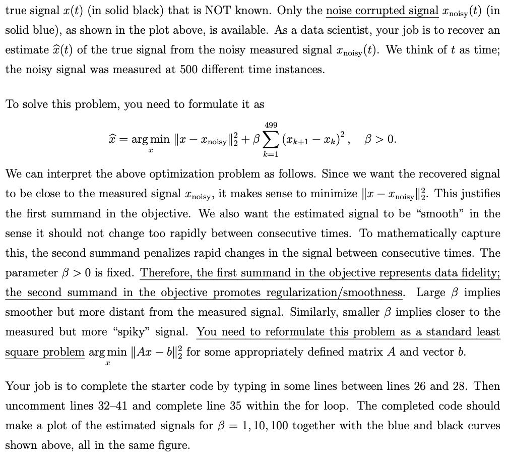
Estimate the true signal from the measured noisy signal (50 points) 8 6 2 Lo -2 -4 -6 -8 50 100 150 200 300 350 400 450 500 250 t true signal x(t) (in solid black) that is NOT known. Only the noise corrupted signal 0. C k=1 We can interpret the above optimization problem as follows. Since we want the recovered signal to be close to the measured signal Xnoisy, it makes sense to minimize || 2 Znoisy ||2. This justifies the first summand in the objective. We also want the estimated signal to be smooth in the sense it should not change too rapidly between consecutive times. To mathematically capture this, the second summand penalizes rapid changes in the signal between consecutive times. The parameter B > 0 is fixed. Therefore, the first summand in the objective represents data fidelity; the second summand in the objective promotes regularization/smoothness. Large B implies smoother but more distant from the measured signal. Similarly, smaller implies closer to the measured but more spiky" signal. You need to reformulate this problem as a standard least square problem arg min || Ax 6||2 for some appropriately defined matrix A and vector b. 2 Your job is to complete the starter code by typing in some lines between lines 26 and 28. Then uncomment lines 3241 and complete line 35 within the for loop. The completed code should make a plot of the estimated signals for B = 1, 10, 100 together with the blue and black curves shown above, all in the same figure. Estimate the true signal from the measured noisy signal (50 points) 8 6 2 Lo -2 -4 -6 -8 50 100 150 200 300 350 400 450 500 250 t true signal x(t) (in solid black) that is NOT known. Only the noise corrupted signal 0. C k=1 We can interpret the above optimization problem as follows. Since we want the recovered signal to be close to the measured signal Xnoisy, it makes sense to minimize || 2 Znoisy ||2. This justifies the first summand in the objective. We also want the estimated signal to be smooth in the sense it should not change too rapidly between consecutive times. To mathematically capture this, the second summand penalizes rapid changes in the signal between consecutive times. The parameter B > 0 is fixed. Therefore, the first summand in the objective represents data fidelity; the second summand in the objective promotes regularization/smoothness. Large B implies smoother but more distant from the measured signal. Similarly, smaller implies closer to the measured but more spiky" signal. You need to reformulate this problem as a standard least square problem arg min || Ax 6||2 for some appropriately defined matrix A and vector b. 2 Your job is to complete the starter code by typing in some lines between lines 26 and 28. Then uncomment lines 3241 and complete line 35 within the for loop. The completed code should make a plot of the estimated signals for B = 1, 10, 100 together with the blue and black curves shown above, all in the same figure