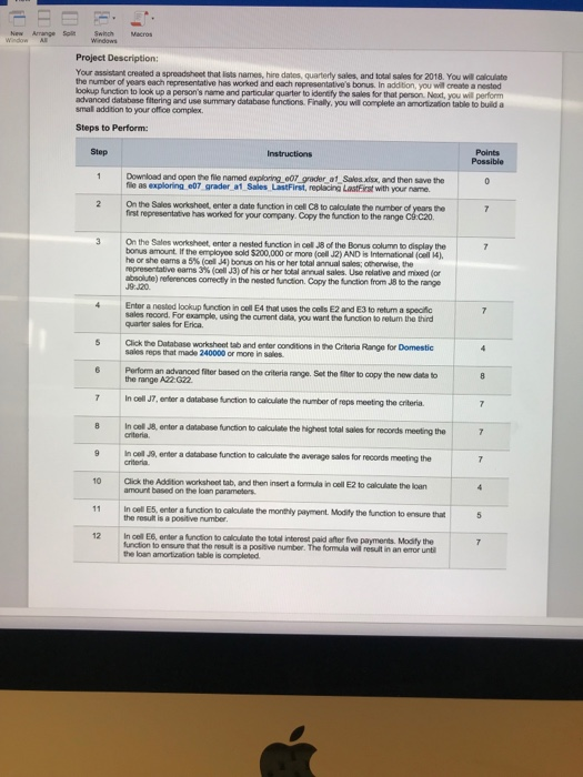
New Arrange Spl Swinch Macros Windows Project Description: Your assistant created a spreadsheet that lists names, hire dates, quarterly sales, and total sales for 2018. You will calculato the number of years each representative has worked and each representative's bonus. In addtion, you will create a nested ookup function advanced database fitering and use summary database functions. Finally, you will complete an amorizaion table to build a small addition to your office complex. to look up a person's name and particular quarter to idenefy the sales for that person. Next, you will perform Steps to Perform: Step Points Possible 1 Download and open the file named exploring e07 grader at Sales.xisx, and then save the fie as exploring e07 grader a1 Sales LastFirst, replacing LastEirst with your name. 2 On the Sales worksheet, enter a date function in cell C8 to caloulate the number of years the first representative has worked for your company. Copy the function to the range C9 C20 3 On the Sales worksheet, enter a nested function in cell J8 of the Bonus column to display the bonus amount. If the empkoyee sold $200,000 or more (cell 12) AND is Intemational (celil ) hear she earns a 5% (cel A) tous on his or her total annual sales; one wise, the represe tative earns 3% (oel J3)ofhs or her total anal sales. Use relative and mixed (or absolute) references comecty in the nested function.Copy the function from J8 to the range 4 Enter a nested lookup function in cell E4 that uses the cells E2 and E3 to retum a specifc sales reoord. For example, using the current data, you want the function to relum the third quarter sales for Erica Click the Database worksheet tab and enter conditions in the Citeria Range for Domestic sales reps that made 240000 or more in sales. Perform an advanced fiter based on the criteria the range A22 G22 range. Set the ther to copy the new dats to In cell J7, enter a database function to calculate t the number of reps meeting the criteria 8 In cell J8, enter a database function to calaulabe the highest t total sales for records meeting the In cell J9, enter a database function to calculate the average sales for records meeting the 10 Click the Addition worksheot tab, and then insert a formula in cell E2 to calculate the loan 11 In cell E5, enter a function to calculate the monthly payment. Modity the function to ensure that 12 In cell E6, enter a function to caloulate the total interest paid after five payments. Modify the amount based on the loan parameters. the result is a positive number function to ensure that the resut is a the loan amortization table is completed positive number. The fomula will result in an eor unti