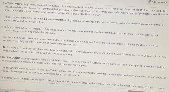
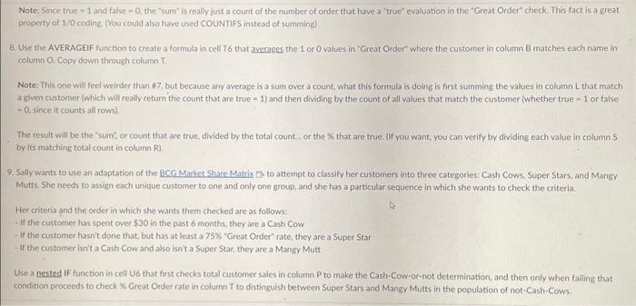
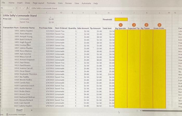
Note: Since true = 1 and false -0 , the "sum" is really just a count of the number of order that have a "true" evaluation in the "Great Order" check. This fact is a great property of 1/0 coding. (You could also have used COUNTIFS instead of summing) 8. Use the AVERAGEIF function to create a formula in cell T6 that averages the 1 or 0 values in "Great Order" where the customer in column B matches each name in column O, Copy down through column T. Note: This one will feel weirder than 47 , but because any average is a sum over a count, what this formula is doing is first summing the values in column L that mateh a given customer (which will really retum the count that are true =1 ) and then dividing by the count of all values that match the customer (whether true =1 or false -0, since it counts all rows) The result will be the "sum; or count that are true, divided by the total count... or the % that are true. (If you want, you can verify by dividing each value in column $ byits matching total count in column R]. 9. Sally wants to use an adaptation of the BCG Markel Share Matrix to to attempt to classify her customers into three categories: Cash Cows, Super Stars, and Mangy Mutts She sheeds to assign each unique customer to one and only one group, and she has a particular sequence in which she wants to check the criteria. Her criteria and the order in which she wants them checked are as follows: - If the customer has spent over $30 in the past 6 months, they are a Cash Cow - If the customer hasn't done that, but has at least a 75% "Great Order" rate, they are a Super 5 tar - If the customer isn't a Cash Cow and also isn't a Super Star, they are a Mangy Mutt Use a nested If function in cell 46 that first checks total customer sales in column P to make the Cash-Cow-or-not determination, and then only when failing that condition proceeds to check \$ Great Order rate in column T to distinguish between Super Stars and Mangy Mutts in the population of not-Cash-Cows. Fle Home Insert Draw Page Layout Formulas Data Rowiew View Automate Help A1. fx title sallys tembnadestand Little Sally's Lemonade Stand Price Lint: Lemonade 53.00 D. E G. H. ). Sweet Tea 5250 Threshold: Transaction Num Cusamer Name Purchase Date Item Ordered Quantity Sale Amount Mip Amount Total Aint Big Spender Expected Thp Bic Hipper Great Order 1001 lulictalionden 1002 lliana Malone 1003 Amivati Young 1004 Kalel Erickson 1005 Wuph flussell 1006 Esteban Xert 1007 Julieta Harden 100a tisna Malone 1009 Ayla Sancher 1010 Macy Cartoll 1011 Armani ferguson 1012 Javi Brovo 1013 Opal Bowes 1014 Joanna Carrell 1015 Oscar flacer 1016 Stephanie Thornton 1017 Sky Padaa 1018 Wetio Holfors 1019 Camila Ruiu 1020 Esperanza leach 1021 Mestin Hortoel 1022 tiodie Dixon 1023 Amaris Crus 1024 Nathanlei Beluan 1025 Rienata Richatd 1026 Cain Harrell 1027 Julieta Hayden | Sheet1 + 4. A 'Great Order" in Sally's estimation is an individual order that either spends a lot or tips a lot. Use a combination of the If function and OR function in cell L6 to check both the Big Spender and Big Tipper true/false logical values and see if either one was true for the given order. Your. "logical test" parameter in your IF functio should be a nested OR function that checks whether "Big Spender" is true or "Big Tipper" is true," Setup your function to return a value of 1 if true and 0 if false (using these numeric codings of the boolean true/fake values is a common aiternative, and will be useful later) Copy down through column L. 5. In the right-hand side of the spreadsheet. Sally has de-duplicated her data by customer name so she can summarize the data for each unique customer that purchased something in the period of January to June. Use the SUMIF function to create a formula in cell P6 that sums the sale amounts in column F when the customer's name in column B matches each unique customer record Sally has entered in column O. Do the same thing for tips. Tip: If you are clever with your use of relative and absolute references to the various columns you need to add and check for name matches in, vou can write a single formula in P6 that can be copied both down that column and over to Q Use the COUNTIF function to create a formula in cell R6 that counts how many times each customer made a purchase in the 6 -month period captured in this data. You can just check the transaction records for the number of times each name appears. Use the SUMIF functon to create a formula in cell 56 that sums up the 1 or 0 values (coding for true or false) you prepared previously under "Great Order" where the customer in column 8 matches each name in column O, Copy down the column. Note: Since true +1 and false =0, the "sum" is really lust a count of the number of order that have a "true" evaluation in the "Great Order" check. This fact is a great Dally has gone back to her hand-tabulated transaction records for January through June of this year in order to do some customer-level analysis to supplement the nonthly summary analysis you did for her in Assignment 2 . This time, she wants to be able to classify each individual order she recorded based on the amount of the firect sale and the amount of the tip. This assignment is to be completed in Excel, with the deliverable being an uploaded worksheet with your formulas and fesporises filled in. There are 9 elements on the preadsheet, each worth 5 points, with 5 additional points for overall accuncy/cleanliness of the work. Note: For this assigrment in particular, there will be many different ways in which the essential result requested by each prompt could be calculated using different unctions or calculation approaches, Please use the formulas indicated so you gain practice with all methods. preadsheet: istructions for individual required elements follow: 1. A "Big Spender" is a category Sally uses to describe individual orders with a sale amount (exclusive of tip) greater than or equal to $9.00. Enter this threshold as a constant in the indicated cell, and then create a formula in cell 16 at the top of the transaction data that uses a simple A-B style comparison operator (your operator won't be just an equal sign) in Excel to return a true or false logical value for each order. Copy down through column 1. 2. The tip that Sally expects to recelve for any given order depends on the order quantity. The relationship is Q-1:\$1.00, 2: $1.50,3:$2.00,4:$2.50,5:$3.00, Create a formula in cell 16 that uses a CHOOSE function that uses quantity for the "index number" parameters, and then selects the correct expected tip value from the schedule given to you by Sally (the corresponding dollar tip values are the "value" parameters), Copy down through column J. 3. A 'Big Tipper is a category Sally uses to describe individual orders with a tig amount greater than the expected tip for the quantity of drinks ordered. Use the If function in cell K6 to compare the actual tip received to the calculated expected tip from a 2 above. Setup your function to return a true or false logical value. Copy down through column K