Only need help with requirements 4,5,6 please!

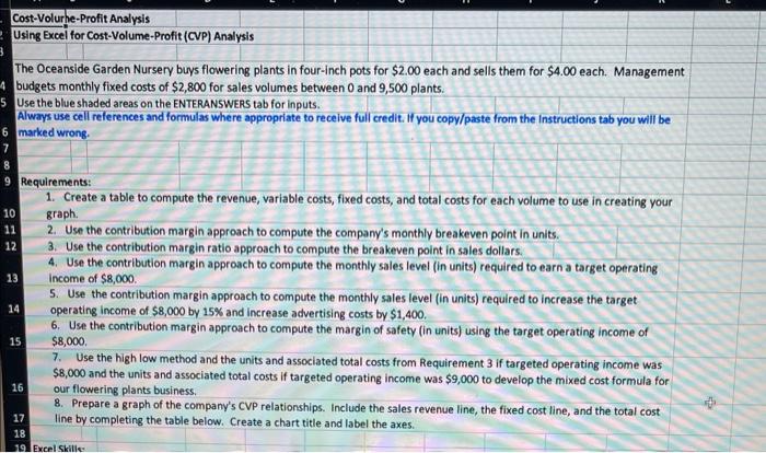
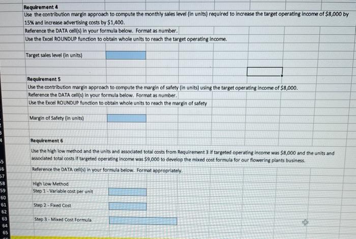
Cost-Volurhe-Profit Analysis Using Excel for Cost-Volume-Profit (CVP) Analysis The Oceanside Garden Nursery buys flowering plants in four-inch pots for $2.00 each and sells them for $4.00 each. Management budgets monthly fixed costs of $2,800 for sales volumes between 0 and 9,500 plants. Use the blue shaded areas on the ENTERANSWERS tab for inputs. Always use cell references and formulas where appropriate to receive full credit. If you copy/paste from the Instructions tab you will be marked wrong. Requirements: 1. Create a table to compute the revenue, variable costs, fixed costs, and total costs for each volume to use in creating your graph. 2. Use the contribution margin approach to compute the company's monthly breakeven point in units. 3. Use the contribution margin ratio approach to compute the breakeven point in sales dollars. 4. Use the contribution margin approach to compute the monthly sales level (in units) required to earn a target operating income of $8,000. 5. Use the contribution margin approach to compute the monthly sales level (in units) required to increase the target operating income of $8,000 by 15% and increase advertising costs by $1,400. 6. Use the contribution margin approach to compute the margin of safety (in units) using the target operating income of $8,000. 7. Use the high low method and the units and associated total costs from Requirement 3 if targeted operating income was $8,000 and the units and associated total costs if targeted operating income was $9,000 to develop the mixed cost formula for our flowering plants business. 16 . 8r. Prepare a graph of the company's CVP relationships. Include the sales revenue line, the fixed cost line, and the total cost line by completing the table below. Create a chart title and label the axes. Requirement 4 Use the contribution margin approach to compute the monthly sales level (in units) required to increase the target operating income of $8,000 by 15% and increase advertising costs by $1,400. Reference the DATA cell(s) in your formula below. Format as number. Use the Excel ROUNDUP function to obtain whole units to reach the target operating income. \begin{tabular}{l} Target sales level (in units) \\ \hline \\ Requirement 5 \\ Use the contribution margin approach to compute the mar \\ Reference the DATA cell(s) in your formula below. Format \\ Use the Excel ROUNDUP function to obtain whole units to rea \\ Margin of Safety (in units) \end{tabular} Requirement 6 Use the high low method and the units and associated total costs from Requirement 3 if targeted operating income was $8,000 and the units and associated total costs if targeted operating income was $9,000 to develop the mixed cost formula for our flowering plants business. Relerence the DATA cell(s) in your formula below. Format appropriately. High Low Method Step 1 - Variable cost per unit Step 2-Fixed Cost Step 3 - Mbed Cost Formula