

Question: Open e09m1Sales and save it as e09m1Sales_LastFirst Group the five regional worksheets and complete the following steps: Insert a new row above row 1 of
- Open e09m1Sales and save it as e09m1Sales_LastFirst
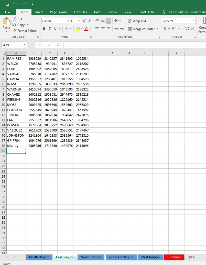
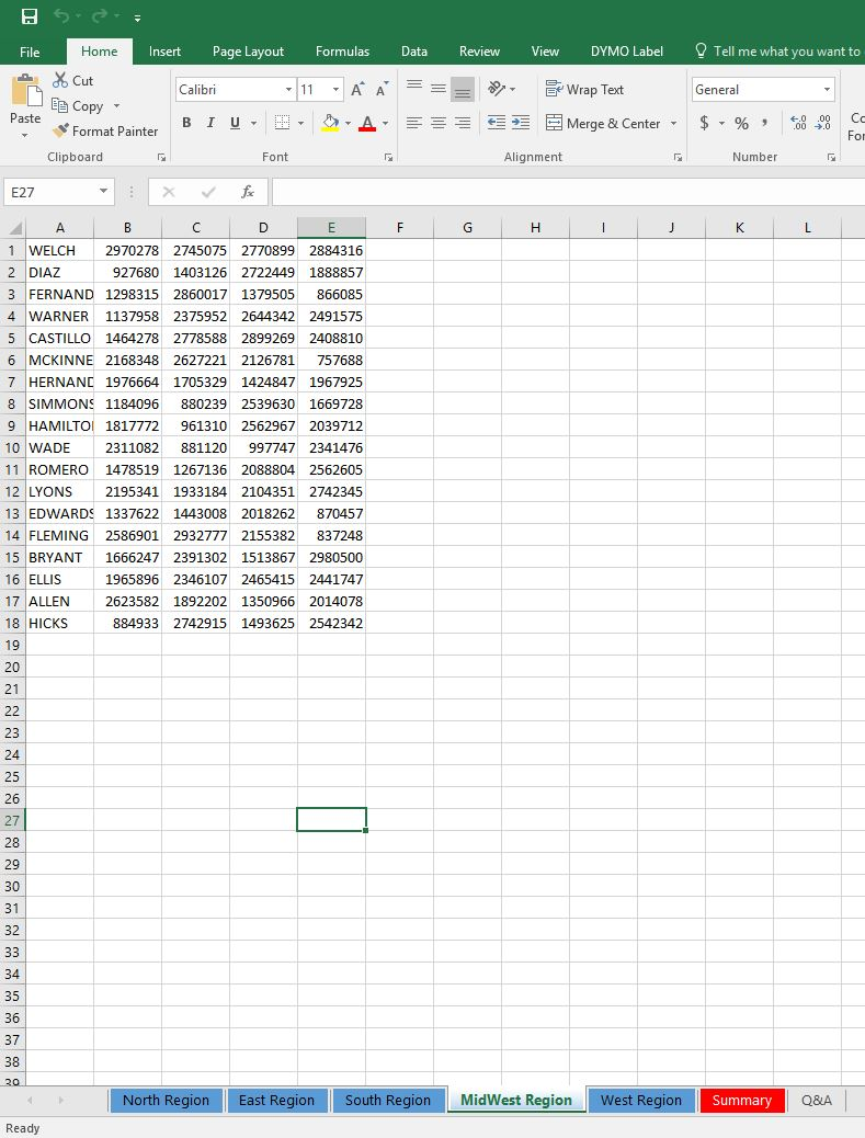
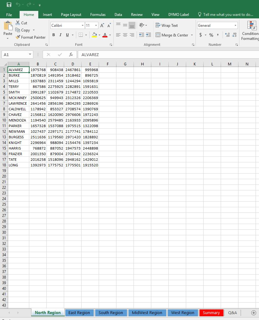
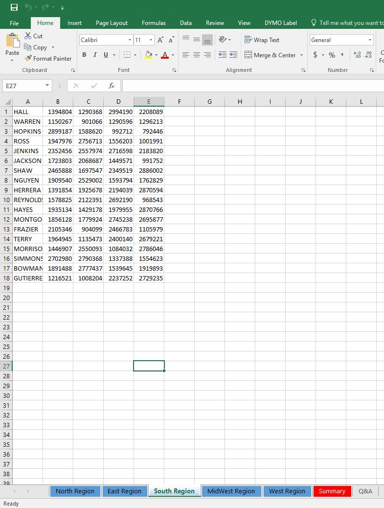
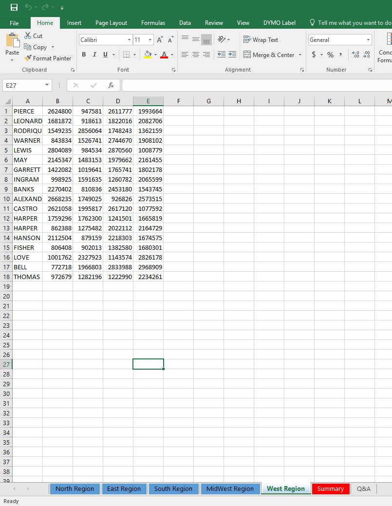
- Group the five regional worksheets and complete the following steps:
- Insert a new row above row 1 of the existing data. Type Agent in cell A1. Apply the Heading 2 Style in the styles group on the home tab.
- Type Qtr1 in cell B1. Use the fill handle to add Qtr2-Qtr4 in cells C1:E1. Apply the Heading 3 Style and apply center horizontal alignment in cells B1:E1
- Type Total in cell F1. Apply the Heading 2 style and horizontal center alignment.
- Click cell F2, type =SUM(B2:F2), and press Enter. Use the fill handle to complete the summary information to the range B3:B19
- Keep the five worksheets grouped (not including the Summary sheet) and complete the following steps:
- Type Total in cell A20. In cell B20, insert a function to total Qtr1 sales. Copy the function to the range C20:F20.
- Format the ranges B2:F2 and B20:F20 with Accounting Number Format and zero decimal places.
- Format range B3:F19 with comma style and zero decimal places.
- Add top and double bottom borders to cells B20:F20
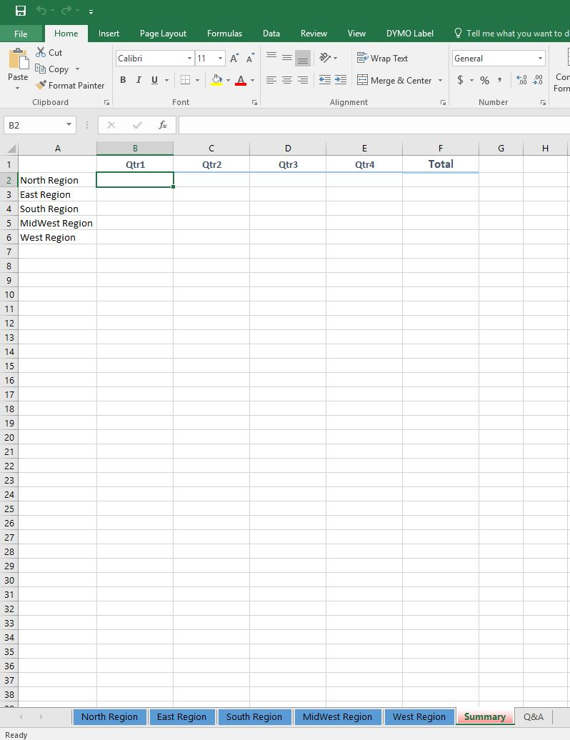
- Ungroup the worksheets and click the Summary sheet tab
- Build formulas with 3-d references by completeing the following steps:
- Click cell B2 and enter a formula that refers to cell B20 in the North region worksheet
- Click cell B3 and enter a formula that refers to cell B20 in the East Region worksheet
- Click cell B4 and enter a formula that refers to cell B20 in the South region worksheet
- Click cell B5 and enter a formula that refers to cell B20 in the Midwest region worksheet
- Click cell B6 and enter a formula that refers to cell B20 in the West Region worksheet.
- Select range B2:B6 and copy the formulas to the range C2:F20
- Apply Accounting Number Format with zero decimal places to the range B2:F2 and Comma Style with zero decimal places to the range B3:F26. Adjust the column widths if they are too narrow to display the formula results.
- Create a hyperlink to create a ScreenTip such as Click to see North Region Sales.
- Set a Watch Window to watch the formulas in the range B2:F6 on the summary sheet.
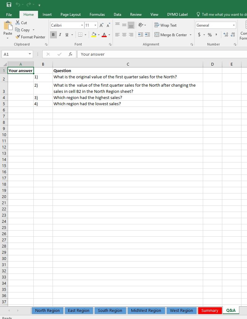
- Use the data in the summary sheet to answer the summary questions 1,3, and 4 in the Q&A sheet.
- Click the North Region Sheet tab, change the value in Cell B2 to 3,000,000 and observe the changes in the Watch Window. Got to the Q&A Sheet and answer question 2.
- Create a footer with your name on the left, the sheet name code in the center and the file name code on the right side of the summary and Q&A sheets.
Step by Step Solution
There are 3 Steps involved in it
1 Expert Approved Answer
Step: 1 Unlock

Question Has Been Solved by an Expert!
Get step-by-step solutions from verified subject matter experts
Step: 2 Unlock
Step: 3 Unlock