• Open our practice workbookhttps://media.gcflearnfree.org/content/56438d60ca7fad0d9cc80512_11_11_2015/excel2016_morepivottables_practice.xlsx
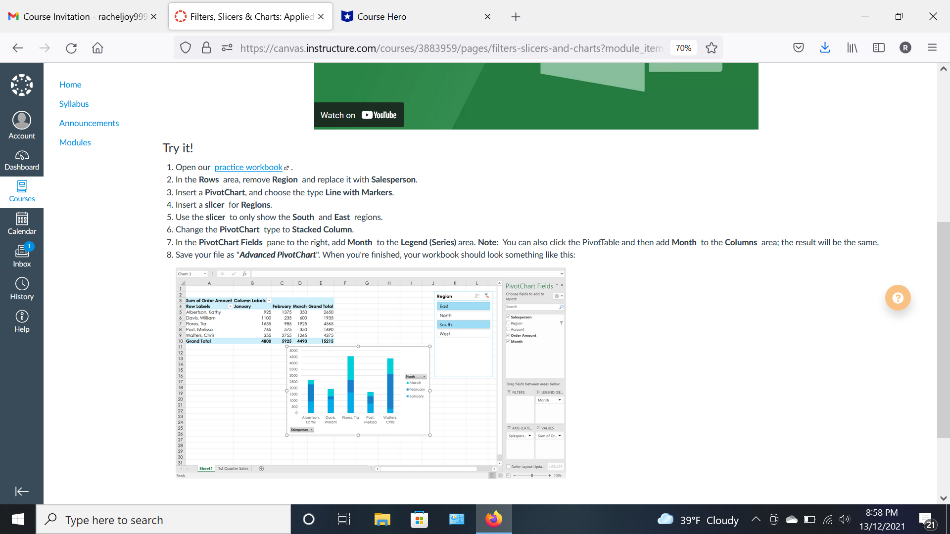
• In the Rows area, remove Region and replace it with Salesperson.
• Insert a PivotChart, and choose the type Line with Markers.
• Insert a slicer for Regions.
• Use the slicer to only show the South and East regions.
• Change the PivotChart type to Stacked Column.
• In the PivotChart Fields pane to the right, add Month to the Legend (Series) area. Note: You can also click the PivotTable and then add Month to the Columns area; the result will be the same.
• Save your file as "Advanced PivotChart". When you're finished, your workbook should look something like this:

M Course Invitation - racheljoy999 X Filters, Slicers & Charts: Applied X Course Hero X + X O 8 . https://canvas.instructure.com/courses/3883959/pages/filters-slicers-and-charts?module_item 70% OLIN BRE Home Syllabus Watch on Youtube Announcements Account Modules Try it! Dashboard 1. Open our practice workbook . 2. In the Rows area, remove Region and replace it with Salesperson. 3. Insert a PivotChart, and choose the type Line with Markers. Courses 4. Insert a slicer for Regions. 88: 5. Use the slicer to only show the South and East regions. Calendar 6. Change the PivotChart type to Stacked Column. 7. In the PivotChart Fields pane to the right, add Month to the Legend (Series) area. Note: You can also click the PivotTable and then add Month to the Columns area; the result will be the same. 8. Save your file as "Advanced PivotChart". When you're finished, your workbook should look something like this: Inbox Chart 1 C D G PivotChart Fields . History Region choose fields to add to ? 3 Sum of Order Amount Column Labels 4 Row Labels January February March Grand Total East 5 Albertson Kathy 925 1375 350 2650 6 Davis, William 1 100 235 1655 985 600 1935 North Salesperson 7 Flores, Tia 4565 South Region Help 8 Post, Melissa 765 575 1690 Account 9 Walters, Chris 355 2755 1265 West Order Amount 10 Grand Total 4800 5925 15215 Month 11 1000 3500 30 00 Month 250 March Drag fields between areas below. 2000 February O January Y FILTERS LEGEND (SE Month Jbertson, Davis. Flores, Tia Melissa Chris" alesperson . AXIS (CATE. E VALUES Salespers. * Sum of Or_ Sheet1 1st Quarter Sales Defer Layout Upda.. UPDATE Ready 100% K 8:58 PM Type here to search O 39.F Cloudy 13/12/2021 721