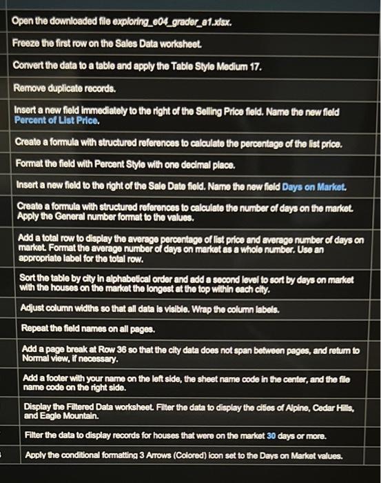
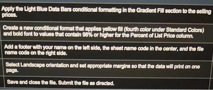
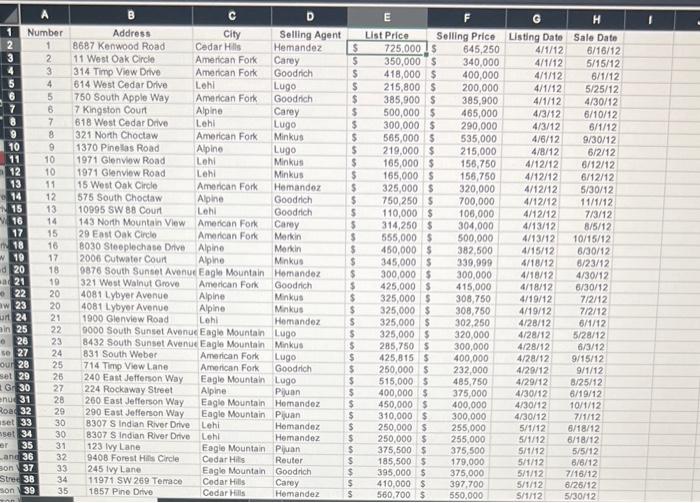
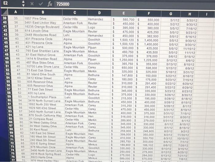
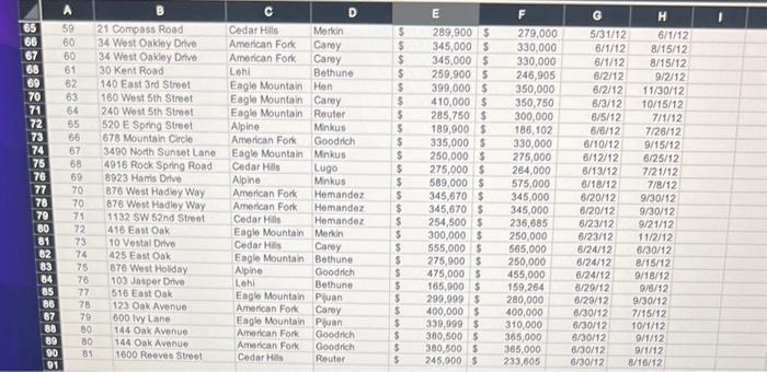
Open the downloaded file exploring_e04_grader_a1. x dsx. Freeze the first row on the Sales Data worksheet. Convert the data to a table and apply the Table Style Medlum 17. Remove duplicate records. Insert a new field immediately to the right of the Selling Price field. Name the new field Percent of Llst Price. Create a formula with structured references to calculate the percentage of the list price. Format the field with Percent Style with one decimal place. Insert a new field to the right of the Sale Date field. Name the new field Days on Market. Create a formula with structured references to calculate the number of days on the market. Apply the General number format to the values. Add a total row to display the average percentage of list price and average number of days on market. Format the average number of days on markot as a whole number. Use an appropriate label for the total row. Sort the table by cily in alphabetical order and add a socond lovel to sort by days on maket with the houses on the market the longest at the top within each elily. Adjust column widths so that all data is visible. Wrap the column labels. Repeat the field names on all pages. Add a page break at Row 36 so that the cily data does not span between peges, and retum to Normal view, if necessary. Add a footer with your name on the left side, the sheet name code in the center, and the flle name code on the right side. Display the Filtered Data worksheet. Filter the data to display the cities of Apine, Cedar Hills, and Eagle Mountain. Filier the data to display records for houses that were on the market 30 days or more. Aoply the conditional formatting 3 Arrows (Colored) icon set to the Davs on Market values. Apply the Light Blue Data Bars conditional formating in the Gradient Fill section to the selling prices. Create a new condilional format that applies yellow fill (fourth color under Standard Colors) and bold font to values that contain 98% or higher for the Percent of List Price column. Add a footer with your name on the left side, the sheet name code in the center, and the file name code on the right side. Select Landscape orientation and set appropriate margins so that the data will print on one page. Save and close the file. Submit the file as directed. Open the downloaded file exploring_e04_grader_a1. x dsx. Freeze the first row on the Sales Data worksheet. Convert the data to a table and apply the Table Style Medlum 17. Remove duplicate records. Insert a new field immediately to the right of the Selling Price field. Name the new field Percent of Llst Price. Create a formula with structured references to calculate the percentage of the list price. Format the field with Percent Style with one decimal place. Insert a new field to the right of the Sale Date field. Name the new field Days on Market. Create a formula with structured references to calculate the number of days on the market. Apply the General number format to the values. Add a total row to display the average percentage of list price and average number of days on market. Format the average number of days on markot as a whole number. Use an appropriate label for the total row. Sort the table by cily in alphabetical order and add a socond lovel to sort by days on maket with the houses on the market the longest at the top within each elily. Adjust column widths so that all data is visible. Wrap the column labels. Repeat the field names on all pages. Add a page break at Row 36 so that the cily data does not span between peges, and retum to Normal view, if necessary. Add a footer with your name on the left side, the sheet name code in the center, and the flle name code on the right side. Display the Filtered Data worksheet. Filter the data to display the cities of Apine, Cedar Hills, and Eagle Mountain. Filier the data to display records for houses that were on the market 30 days or more. Aoply the conditional formatting 3 Arrows (Colored) icon set to the Davs on Market values. Apply the Light Blue Data Bars conditional formating in the Gradient Fill section to the selling prices. Create a new condilional format that applies yellow fill (fourth color under Standard Colors) and bold font to values that contain 98% or higher for the Percent of List Price column. Add a footer with your name on the left side, the sheet name code in the center, and the file name code on the right side. Select Landscape orientation and set appropriate margins so that the data will print on one page. Save and close the file. Submit the file as directed