optimization

here's the information from the textbook including iterations 1 & 2. so i need help with the next 2 iterations.

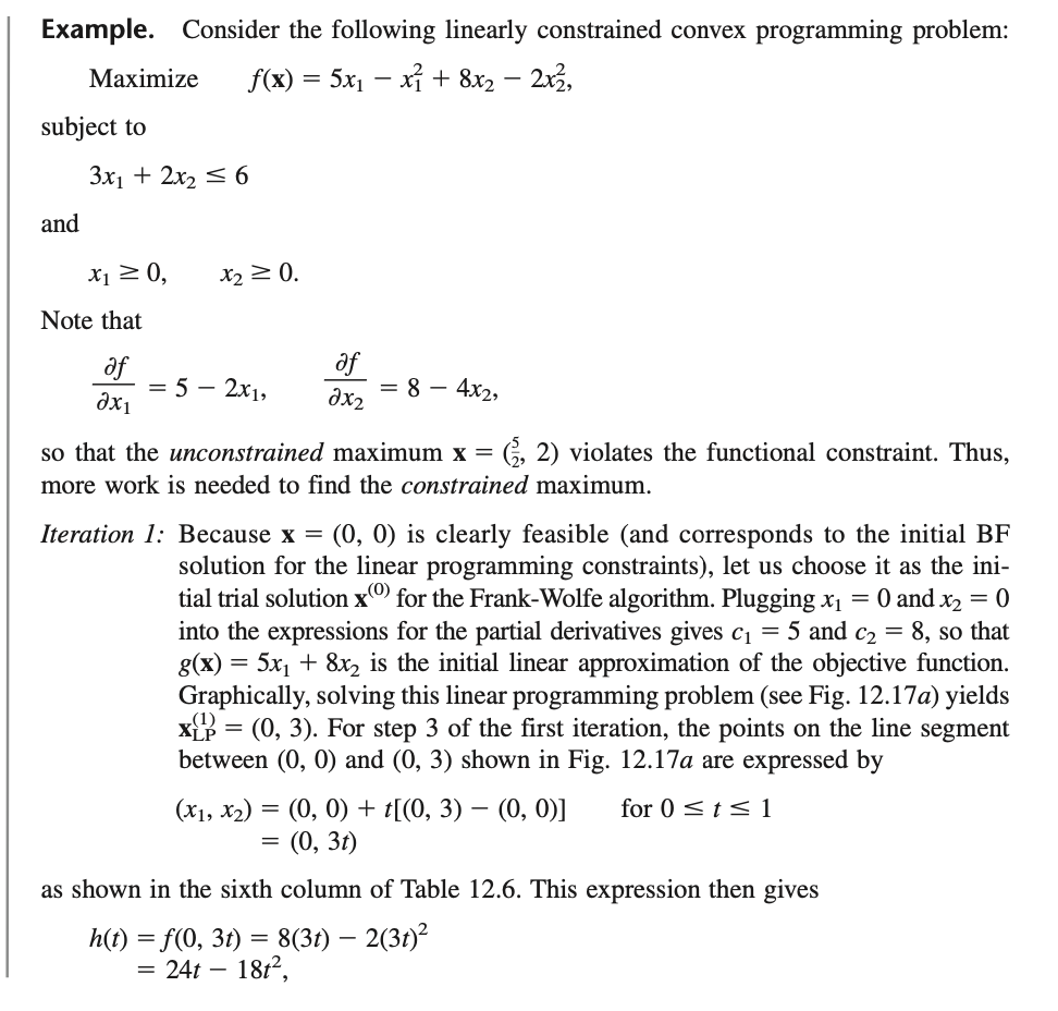
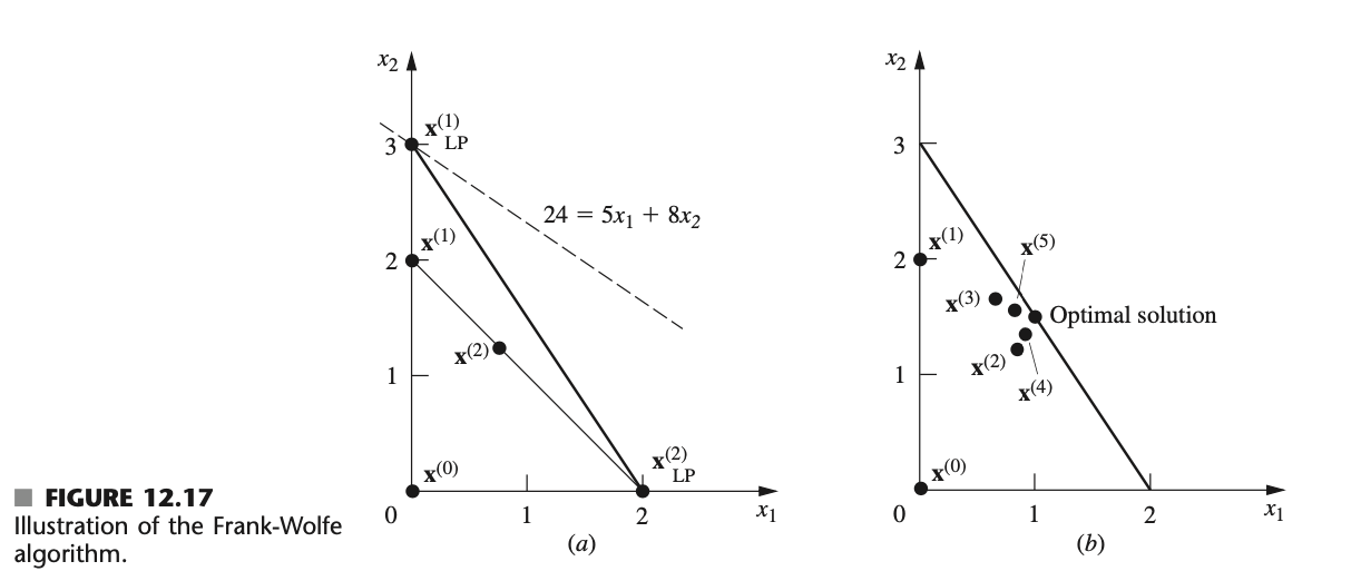
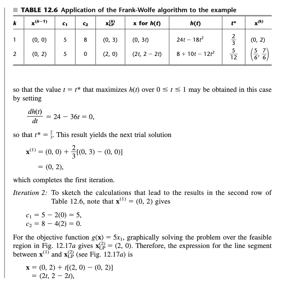
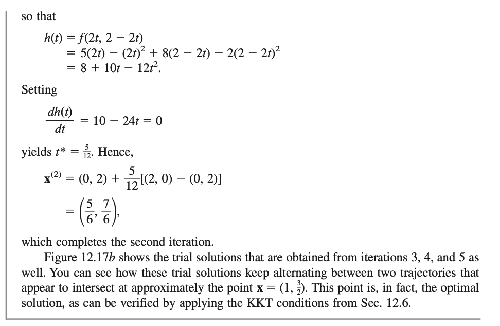
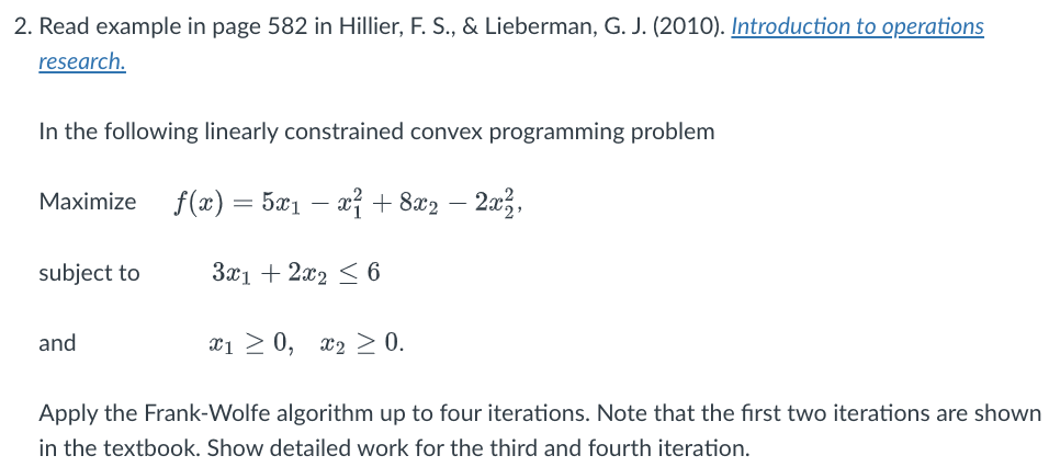
2. Read example in page 582 in Hillier, F. S., \& Lieberman, G. J. (2010). Introduction to operations research. In the following linearly constrained convex programming problem Maximize f(x)=5x1x12+8x22x22, subject to 3x1+2x26 and x10,x20 Apply the Frank-Wolfe algorithm up to four iterations. Note that the first two iterations are shown in the textbook. Show detailed work for the third and fourth iteration. Maximize f(x)=5x1x12+8x22x22, subject to 3x1+2x26 and x10,x20. Note that x1f=52x1,x2f=84x2, so that the unconstrained maximum x=(25,2) violates the functional constraint. Thus, more work is needed to find the constrained maximum. Iteration 1: Because x=(0,0) is clearly feasible (and corresponds to the initial BF solution for the linear programming constraints), let us choose it as the initial trial solution x(0) for the Frank-Wolfe algorithm. Plugging x1=0 and x2=0 into the expressions for the partial derivatives gives c1=5 and c2=8, so that g(x)=5x1+8x2 is the initial linear approximation of the objective function. Graphically, solving this linear programming problem (see Fig. 12.17a) yields xLP(1)=(0,3). For step 3 of the first iteration, the points on the line segment between (0,0) and (0,3) shown in Fig. 12.17a are expressed by (x1,x2)=(0,0)+t[(0,3)(0,0)] for 0t1 =(0,3t) as shown in the sixth column of Table 12.6. This expression then gives h(t)=f(0,3t)=8(3t)2(3t)2 FIGURE 12.17 Illustration of the Frank-Wolf algorithm. TABLE 12.6 Application of the Frank-Wolfe algorithm to the example so that the value t=t that maximizes h(t) over 0t1 may be obtained in this case by setting dtdh(t)=2436t=0, so that t=32. This result yields the next trial solution x(1)=(0,0)+32[(0,3)(0,0)]=(0,2), which completes the first iteration. Iteration 2: To sketch the calculations that lead to the results in the second row of Table 12.6, note that x(1)=(0,2) gives c1=52(0)=5,c2=84(2)=0. For the objective function g(x)=5x1, graphically solving the problem over the feasible region in Fig. 12.17a gives xLP(2)=(2,0). Therefore, the expression for the line segment between x(1) and xLP(2) (see Fig. 12.17a) is x=(0,2)+t[(2,0)(0,2)]=(2t,22t) so that h(t)=f(2t,22t)=5(2t)(2t)2+8(22t)2(22t)2=8+10t12t2 Setting dtdh(t)=1024t=0 yields t=125. Hence, x(2)=(0,2)+125[(2,0)(0,2)]=(65,67), which completes the second iteration. Figure 12.17b shows the trial solutions that are obtained from iterations 3,4 , and 5 as well. You can see how these trial solutions keep alternating between two trajectories that appear to intersect at approximately the point x=(1,23). This point is, in fact, the optimal solution, as can be verified by applying the KKT conditions from Sec. 12.6. 2. Read example in page 582 in Hillier, F. S., \& Lieberman, G. J. (2010). Introduction to operations research. In the following linearly constrained convex programming problem Maximize f(x)=5x1x12+8x22x22, subject to 3x1+2x26 and x10,x20 Apply the Frank-Wolfe algorithm up to four iterations. Note that the first two iterations are shown in the textbook. Show detailed work for the third and fourth iteration. Maximize f(x)=5x1x12+8x22x22, subject to 3x1+2x26 and x10,x20. Note that x1f=52x1,x2f=84x2, so that the unconstrained maximum x=(25,2) violates the functional constraint. Thus, more work is needed to find the constrained maximum. Iteration 1: Because x=(0,0) is clearly feasible (and corresponds to the initial BF solution for the linear programming constraints), let us choose it as the initial trial solution x(0) for the Frank-Wolfe algorithm. Plugging x1=0 and x2=0 into the expressions for the partial derivatives gives c1=5 and c2=8, so that g(x)=5x1+8x2 is the initial linear approximation of the objective function. Graphically, solving this linear programming problem (see Fig. 12.17a) yields xLP(1)=(0,3). For step 3 of the first iteration, the points on the line segment between (0,0) and (0,3) shown in Fig. 12.17a are expressed by (x1,x2)=(0,0)+t[(0,3)(0,0)] for 0t1 =(0,3t) as shown in the sixth column of Table 12.6. This expression then gives h(t)=f(0,3t)=8(3t)2(3t)2 FIGURE 12.17 Illustration of the Frank-Wolf algorithm. TABLE 12.6 Application of the Frank-Wolfe algorithm to the example so that the value t=t that maximizes h(t) over 0t1 may be obtained in this case by setting dtdh(t)=2436t=0, so that t=32. This result yields the next trial solution x(1)=(0,0)+32[(0,3)(0,0)]=(0,2), which completes the first iteration. Iteration 2: To sketch the calculations that lead to the results in the second row of Table 12.6, note that x(1)=(0,2) gives c1=52(0)=5,c2=84(2)=0. For the objective function g(x)=5x1, graphically solving the problem over the feasible region in Fig. 12.17a gives xLP(2)=(2,0). Therefore, the expression for the line segment between x(1) and xLP(2) (see Fig. 12.17a) is x=(0,2)+t[(2,0)(0,2)]=(2t,22t) so that h(t)=f(2t,22t)=5(2t)(2t)2+8(22t)2(22t)2=8+10t12t2 Setting dtdh(t)=1024t=0 yields t=125. Hence, x(2)=(0,2)+125[(2,0)(0,2)]=(65,67), which completes the second iteration. Figure 12.17b shows the trial solutions that are obtained from iterations 3,4 , and 5 as well. You can see how these trial solutions keep alternating between two trajectories that appear to intersect at approximately the point x=(1,23). This point is, in fact, the optimal solution, as can be verified by applying the KKT conditions from Sec. 12.6