$\%$ Parameters T $=4$;$\%$ Defines the Period of T w$0=2*$ pi $/$ T;$\%$ Calculates the fundamental angular frequency t $=-6$:$0\mathrm{.}01$:$6$;$\%$ Creates a time vector ranging from $6$ to $6$ with a step size of $0\mathrm{.}01\%$ Coefficients a$0=3/4$; $\%$ Sets the DC component, representing the average value of the signal over one period an $=$ @$($n$)-1./($pi$*$n$).*$ sin$($pi$*$n$/2)$;$\%$ Formula for an calculated in task $1$ A bn $=$ @$($n$)(1./($pi$*$n$)).*$ cos$($pi$*$n$/2)-2*$cos$($pi$*$n$)+1./($pi$*$n$)$;$\%$ Formula for bn calculated in task $1$ A $\%$ Ideal signal definition x$\_$ideal $=(($t $>=0)$ & $($t t $>=1)$ & $($t $<mtext></mtext><mn>2</mn><mi>)</mi><mi>)</mi>$;$\%$ Defines an ideal signal with amplitude $1$ from $0$ to $1,$ and amplitude $2$ from $1$ to $2\%$ Fourier series approximations for N $=17$ and N $=51$ x$\_$fourier$\_17=$ a$0*$ ones$($size$($t$))$;$\%$ Start with DC component for N$=17$ x$\_$fourier$\_51=$ a$0*$ ones$($size$($t$))$;$\%$ Start with DC component for N$=51\%$ Define piecewise function f$\_$piecewise $=$ @$($t$)(($t $>=0)$ & $($t t $>=1)$ & $($t $<mtext></mtext><mn>2</mn><mi>)</mi><mi>)</mi>$;$\%$ Defines a piecewise function with values $1$ for t $<mtext></mtext><mn>1</mn>$ and $2$ for t Functions to compute Fourier coefficients compute$\_$coefficients $=$ @$($n$)$ deal$(...(2/$ T$)*($integral$($@$($t$)$ f$\_$piecewise$($t$).*$ cos$($n $*$ w$0*$ t$),0,1)+...$ integral$($@$($t$)$ f$\_$piecewise$($t$).*$ cos$($n $*$ w$0*$ t$),1,2)),...(2/$ T$)*($integral$($@$($t$)$ f$\_$piecewise$($t$).*$ sin$($n $*$ w$0*$ t$),0,1)+...$ integral$($@$($t$)$ f$\_$piecewise$($t$).*$ sin$($n $*$ w$0*$ t$),1,2))...)$;$\%$ Inputs the Fourier coefficients for the piecewise function over the interval $[0,2]\%$ Calculate Fourier series for N $=17$ harmonics for n $=1$:$17[$an$,$ bn$]=$ compute$\_$coefficients$($n$)$;$\%$ Inputs the Fourier coefficients for the nth harmonic x$\_$fourier$\_17=$ x$\_$fourier$\_17+$ an $*$ cos$($n $*$ w$0*$ t$)+$ bn $*$ sin$($n $*$ w$0*$ t$)$;$\%$ Adds the nth harmonic to the Fourier series approximation end $\%$ Calculate Fourier series for N $=51$ harmonics for n $=1$:$51[$an$,$ bn$]=$ compute$\_$coefficients$($n$)$;$\%$ Inputs the Fourier coefficients for the nth harmonic x$\_$fourier$\_51=$ x$\_$fourier$\_51+$ an $*$ cos$($n $*$ w$0*$ t$)+$ bn $*$ sin$($n $*$ w$0*$ t$)$;$\%$ Adds the nth harmonic to the Fourier series approximation end $\%$ Plotting figure$(\text{'}$Color$\text{'},$ 'white'$)$;$\%$ Creates a figure with a white background $\%$ Plot the ideal signal plot$($t$,$ x$\_$ideal, $\text{'}$k$\text{'},$ 'LineWidth', $2,$ 'DisplayName', 'Ideal x$($t$)\text{'})$;$\%$ Plots the original ideal signal x$($t$)$ hold on;$\%$ Holds the current plot for further additions $\%$ Plot Fourier series approximations plot$($t$,$ x$\_$fourier$\_17,\text{'}$r$--\text{'},$ 'LineWidth', $1\mathrm{.}5,$ 'DisplayName', 'Fourier Approx $($N$=17)\text{'})$;$\%$ Plots the Fourier series approximation with $17$ harmonics plot$($t$,$ x$\_$fourier$\_51,\text{'}$b$-.\text{'},$ 'LineWidth', $1\mathrm{.}5,$ 'DisplayName', 'Fourier Approx $($N$=51)\text{'})$;$\%$ Plots the Fourier series approximation with $51$ harmonics $\%$ Add labels, legend, title, and grid xlabel$(\text{'}$Time $($t$)\text{'})$; $\%$ Labels the x$-$axis as "Time $($t$)"$ ylabel$(\text{'}$x$($t$)\text{'})$; $\%$ Labels the y$-$axis as $"$x$($t$)"$ title$(\text{'}$Ideal Signal and Fourier Series Approximations'$)$; $\%$ Adds a title displaying the Ideal Signal and Fourier Series Approximations legend$(\text{'}$Location$\text{'},$ 'best'$)$; $\%$ Automatically place the legend grid on; $\%$ Turns on the grid for better visualization axis$([-66-0\mathrm{.}52\mathrm{.}5])$; $\%$ Sets the axis limits for the plot: x from $-6$ to $6$ and y from $-0\mathrm{.}5$ to $2\mathrm{.}5\%$ Add vertical and horizontal reference lines plot$([00],[-0\mathrm{.}52\mathrm{.}5],\text{'}$k$--\text{'},$ 'LineWidth', $0\mathrm{.}5)$; $\%$ Vertical line at t$=0$ plot$([-66],[00],\text{'}$k$--\text{'},$ 'LineWidth', $0\mathrm{.}5)$; $\%$ Horizontal line at x$=0$ hold off;$\%$ Release the plot for further change

Edit the code to plot magnitude and phase spectrum for x$($t$).$ The code has to work $100\%$ Task $2-$ Signal Processing

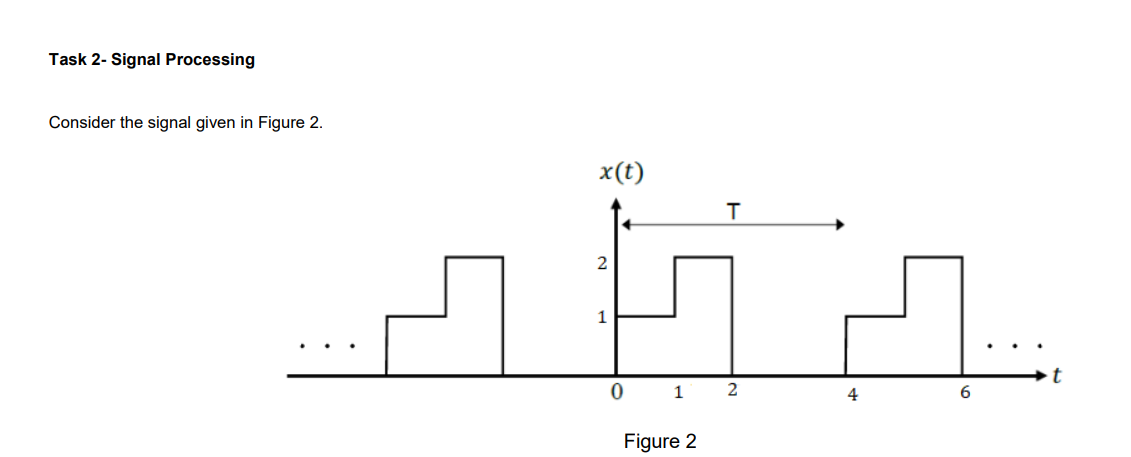
Consider the signal given in Figure $2.$