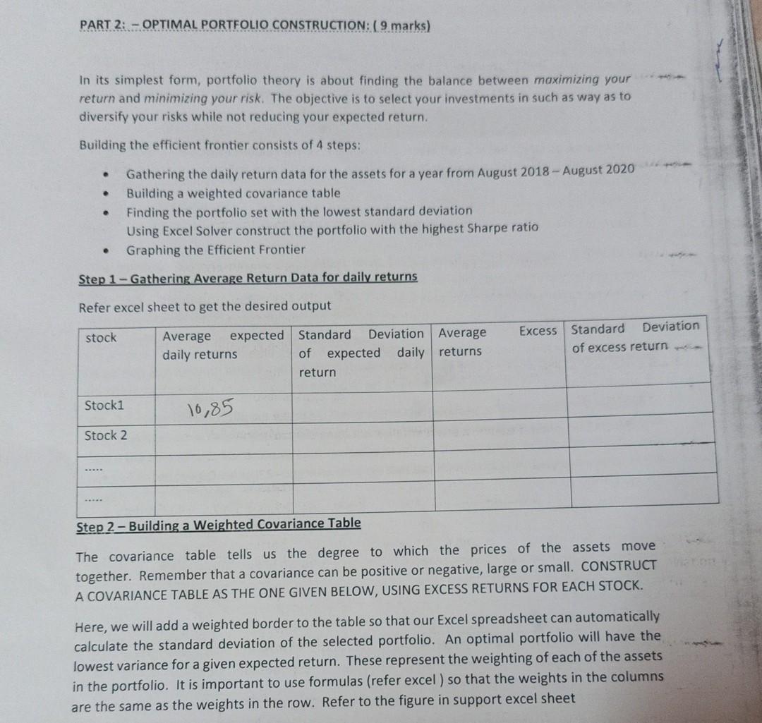
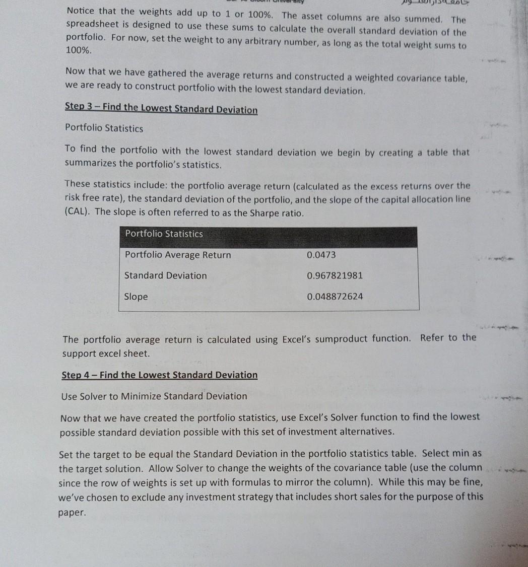
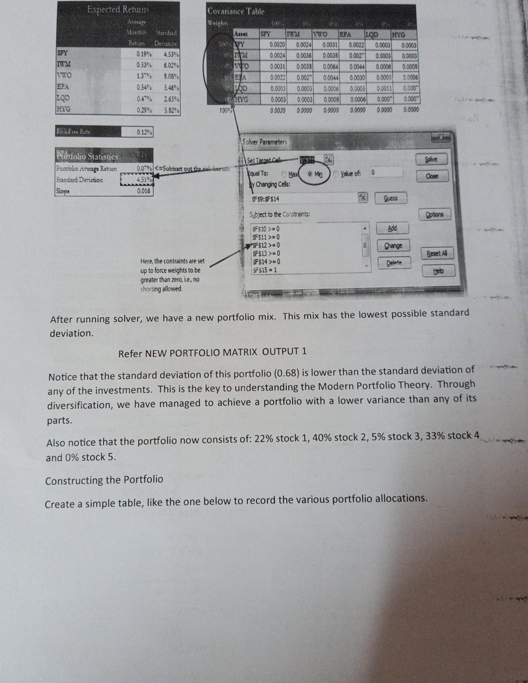
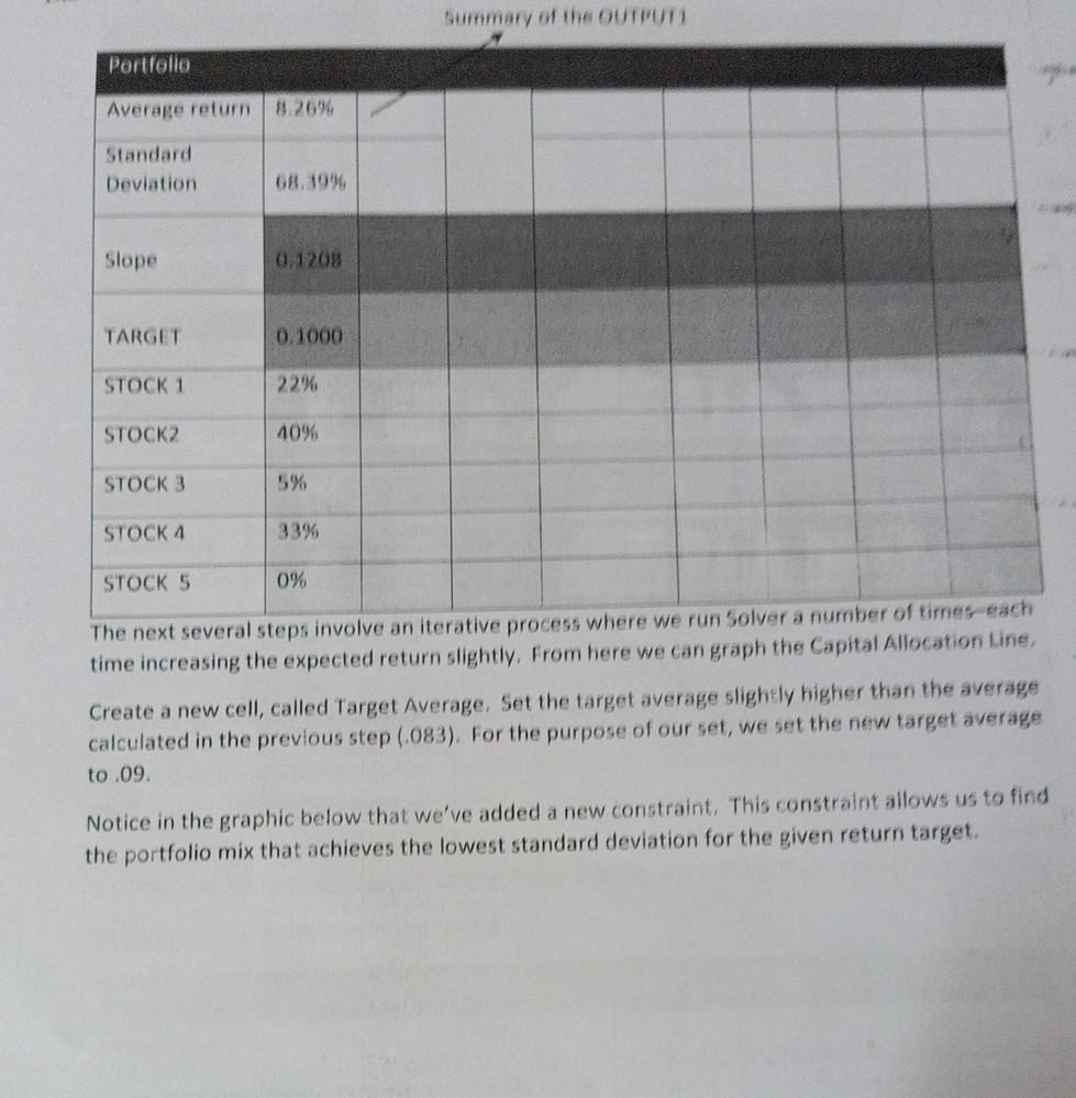
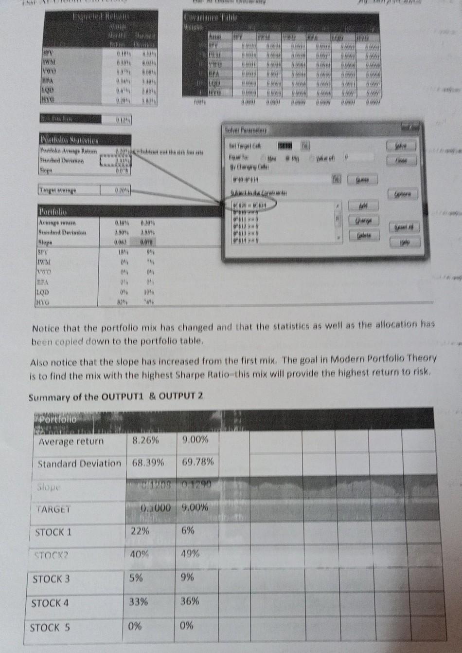
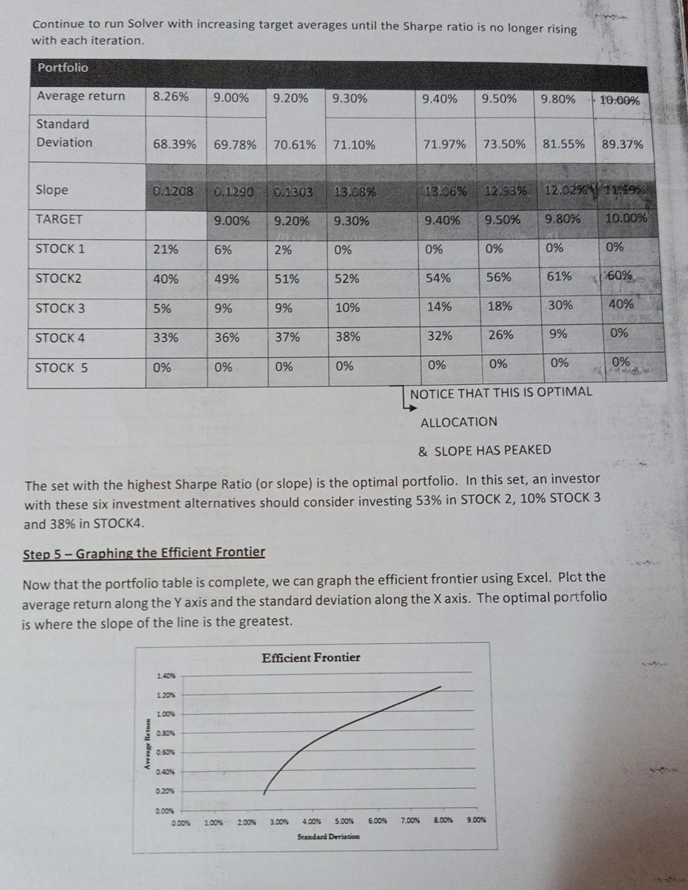
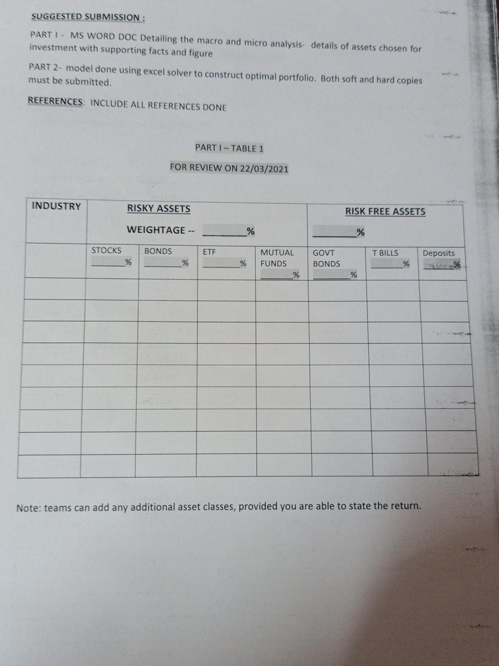
PART 2: - OPTIMAL PORTFOLIO CONSTRUCTION: (9 marks) In its simplest form, portfolio theory is about finding the balance between maximizing your return and minimizing your risk. The objective is to select your investments in such as way as to diversify your risks while not reducing your expected return. Building the efficient frontier consists of 4 steps: Gathering the daily return data for the assets for a year from August 2018 - August 2020 Building a weighted covariance table Finding the portfolio set with the lowest standard deviation Using Excel Solver construct the portfolio with the highest Sharpe ratio Graphing the Efficient Frontier Step 1 - Gathering Average Return Data for daily returns Refer excel sheet to get the desired output stock Average expected Standard Deviation Average daily returns of expected daily returns return Excess Standard Deviation of excess return Stock1 16,85 Stock 2 Step 2 - Building a Weighted Covariance Table The covariance table tells us the degree to which the prices of the assets move together. Remember that a covariance can be positive or negative, large or small. CONSTRUCT A COVARIANCE TABLE AS THE ONE GIVEN BELOW, USING EXCESS RETURNS FOR EACH STOCK. Here, we will add a weighted border to the table so that our Excel spreadsheet can automatically calculate the standard deviation of the selected portfolio. An optimal portfolio will have the lowest variance for a given expected return. These represent the weighting of each of the assets in the portfolio. It is important to use formulas (refer excel) so that the weights in the columns are the same as the weights in the row. Refer to the figure in support excel sheet Notice that the weights add up to 1 or 100%. The asset columns are also summed. The spreadsheet is designed to use these sums to calculate the overall standard deviation of the portfolio. For now, set the weight to any arbitrary number, as long as the total weight sums to 100%. Now that we have gathered the average returns and constructed a weighted covariance table, we are ready to construct portfolio with the lowest standard deviation. Step 3 - Find the Lowest Standard Deviation Portfolio Statistics To find the portfolio with the lowest standard deviation we begin by creating a table that summarizes the portfolio's statistics. These statistics include: the portfolio average return (calculated as the excess returns over the risk free rate), the standard deviation of the portfolio, and the slope of the capital allocation line (CAL). The slope is often referred to as the Sharpe ratio. Portfolio Statistics Portfolio Average Return 0.0473 Standard Deviation 0.967821981 Slope 0.048872624 The portfolio average return is calculated using Excel's sumproduct function. Refer to the support excel sheet. Step 4 - Find the Lowest Standard Deviation Use Solver to Minimize Standard Deviation Now that we have created the portfolio statistics, use Excel's Solver function to find the lowest possible standard deviation possible with this set of investment alternatives. Set the target to be equal the Standard Deviation in the portfolio statistics table. Select min as the target solution. Allow Solver to change the weights of the covariance table (use the column since the row of weights is set up with formulas to mirror the column). While this may be fine, we've chosen to exclude any investment strategy that includes short sales for the purpose of this paper. Standard SPY MWA wo EFA LOD HYG Expected Returns Aretag Manthil Retut Deration 0.19% 4,53 0.33% 6.0296 1.37 8.08% 0.54% 5.46 2.65% 0.29% 5.82% Covariance Table Weight Asset SPY IS PY 0.0020 0. Mar 0.0024 vo 0.0031 ETA 0.0022 HD 0.0003 HYG 0.0003 1004 0.0020 Ivo EPA LOD HYG 0.0024 0.0031 0.0022 0.0003 0.0003 0.0036 0.0039 0.002- 0.0003 0.0003 0.0038 0.0064 0.0044 0.0006 0.0005 0.0021 0.0044 0.0030 0.0003 0.0006 0.0003 0.0006 0.0003 0.0011 0.000 0.0003 0.0005 0.0006 0.0007 0.0001 0.00% 0.00) 0.0000 0.00 0.00 F Free Rate 0.12% Solver Parameters Set Teet.cl 32 ES Solve Puttfolio Statistics Portrolio reage Return Standard Denation Slope 0.0"=0 SF$11 >= 0 F$12 >=0 SF$13 >=0 SF514 >=0 $F$15 = 1 Change Reset AL Delete Help Here, the contraints are set up to force weights to be greater than zero, le, no shorting allowed After running solver, we have a new portfolio mix. This mix has the lowest possible standard deviation. Refer NEW PORTFOLIO MATRIX OUTPUT 1 Notice that the standard deviation of this portfolio (0.68) is lower than the standard deviation of any of the investments. This is the key to understanding the Modern Portfolio Theory. Through diversification, we have managed to achieve a portfolio with a lower variance than any of its parts. Also notice that the portfolio now consists of: 22% stock 1, 40% stock 2,5% stock 3,33% stock 4 and 0% stock 5. Constructing the Portfolio Create a simple table, like the one below to record the various portfolio allocations. Portfolio Average return 8.26% Standard Deviation 68.39% Slope 0.1208 TARGET 0.1000 STOCK 1 22% STOCK2 40% STOCK 3 STOCK 4 STOCK 5 0% The next several steps involve an iterative process where we run Solver a number of times each time increasing the expected return slightly. From here we can graph the Capital Allocation Line, Create a new cell, called Target Average. Set the target average slightly higher than the average calculated in the previous step (083). For the purpose of our set, we set the new target average to .09. Notice in the graphic below that we've added a new constraint, This constraint allows us to find the portfolio mix that achieves the lowest standard deviation for the given return target. THE cual A CY GH 13 WA 8091 PA I LOU DIVO www QU When 14 06 #l Bolver arrested Phatake Arty Hope ARA 00 0201 Portfolio WOWO tre 0 0. wo 3.2013 0,043 181 05 04 0.048 08 IS) 011 01 101 09 LOD (HY Notice that the portfolio mix has changed and that the statistics as well as the allocation has been copied down to the portfolio table, Also notice that the slope has increased from the first mix. The goal in Modern Portfolio Theory is to find the mix with the highest Sharpe Ratio this mix will provide the highest return to risk Summary of the OUTPUTI & OUTPUT 2 Average return 8.26% 9.00% Standard Deviation 68.39% 69.78% Slope OMOS 0 1290 TARGET 0.0000 9.00% STOCK 1 22% 6% STOCK 40% 49% STOCK 3 5% 9% STOCK 4 33% 36% STOCK 5 0% 0% Continue to run Solver with increasing target averages until the Sharpe ratio is no longer rising with each iteration. Portfolio Average return 8.26% 9.00% 9.20% 9.30% 9.40% 9.50% 9.80% 10.00% Standard Deviation 68.39% 69.78% 70.61% 71.10% 71.97% 73.50% 81.55% 89.37% Slope 0.1208 0.1290 0.1303 13.08% 13.06% 12.98% 12.02% | 11.49% TARGET 9.00% 9.20% 9.30% 9.40% 9.50% 9.80% 10.00% STOCK 1 21% 6% 2% 0% 0% 0% 0% 0% STOCK2 40% 49% 51% 52% 54% 56% 61% 60% STOCK 3 5% 9% 9% 10% 14% 18% 30% 40% STOCK 4 33% 36% 37% 38% 32% 26% 9% 0% 0% STOCK 5 0% 0% 0% 0% 0% 0% 0% NOTICE THAT THIS IS OPTIMAL ALLOCATION & SLOPE HAS PEAKED The set with the highest Sharpe Ratio (or slope) is the optimal portfolio. In this set, an investor with these six investment alternatives should consider investing 53% in STOCK 2, 10% STOCK 3 and 38% in STOCK4. Step 5 - Graphing the Efficient Frontier Now that the portfolio table is complete, we can graph the efficient frontier using Excel. Plot the average return along the Y axis and the standard deviation along the X axis. The optimal portfolio is where the slope of the line is the greatest. Efficient Frontier 100% en Retur 0.50% 0.20% 0.00% 100% 2.00% 3.00% 6.00% 7.00% 8.00% 9.00% 5.00% Standard Deviation SUGGESTED SUBMISSION : PART I - MS WORD DOC Detailing the macro and micro analysis- details of assets chosen for investment with supporting facts and figure PART 2- model done using excel solver to construct optimal portfolio. Both soft and hard copies must be submitted. REFERENCES: INCLUDE ALL REFERENCES DONE PARTI - TABLE 1 FOR REVIEW ON 22/03/2021 INDUSTRY RISKY ASSETS RISK FREE ASSETS WEIGHTAGE -- % % BONDS ETF STOCKS % Deposits % MUTUAL FUNDS % GOVT BONDS T BILLS % % % Note: teams can add any additional asset classes, provided you are able to state the return. FOR FINAL SUBMISSION ECONOMY ANALYSIS REPORT INDUSTRY ANALYSIS REPORT COMPANY ANALYSIS REPORT TABLE -1 Company chosen and weightage PART II - TABLE 1 SUMMARY OF OUTPUT TABLES EFFICIENT FRONTIER GRAPH PART 2: - OPTIMAL PORTFOLIO CONSTRUCTION: (9 marks) In its simplest form, portfolio theory is about finding the balance between maximizing your return and minimizing your risk. The objective is to select your investments in such as way as to diversify your risks while not reducing your expected return. Building the efficient frontier consists of 4 steps: Gathering the daily return data for the assets for a year from August 2018 - August 2020 Building a weighted covariance table Finding the portfolio set with the lowest standard deviation Using Excel Solver construct the portfolio with the highest Sharpe ratio Graphing the Efficient Frontier Step 1 - Gathering Average Return Data for daily returns Refer excel sheet to get the desired output stock Average expected Standard Deviation Average daily returns of expected daily returns return Excess Standard Deviation of excess return Stock1 16,85 Stock 2 Step 2 - Building a Weighted Covariance Table The covariance table tells us the degree to which the prices of the assets move together. Remember that a covariance can be positive or negative, large or small. CONSTRUCT A COVARIANCE TABLE AS THE ONE GIVEN BELOW, USING EXCESS RETURNS FOR EACH STOCK. Here, we will add a weighted border to the table so that our Excel spreadsheet can automatically calculate the standard deviation of the selected portfolio. An optimal portfolio will have the lowest variance for a given expected return. These represent the weighting of each of the assets in the portfolio. It is important to use formulas (refer excel) so that the weights in the columns are the same as the weights in the row. Refer to the figure in support excel sheet Notice that the weights add up to 1 or 100%. The asset columns are also summed. The spreadsheet is designed to use these sums to calculate the overall standard deviation of the portfolio. For now, set the weight to any arbitrary number, as long as the total weight sums to 100%. Now that we have gathered the average returns and constructed a weighted covariance table, we are ready to construct portfolio with the lowest standard deviation. Step 3 - Find the Lowest Standard Deviation Portfolio Statistics To find the portfolio with the lowest standard deviation we begin by creating a table that summarizes the portfolio's statistics. These statistics include: the portfolio average return (calculated as the excess returns over the risk free rate), the standard deviation of the portfolio, and the slope of the capital allocation line (CAL). The slope is often referred to as the Sharpe ratio. Portfolio Statistics Portfolio Average Return 0.0473 Standard Deviation 0.967821981 Slope 0.048872624 The portfolio average return is calculated using Excel's sumproduct function. Refer to the support excel sheet. Step 4 - Find the Lowest Standard Deviation Use Solver to Minimize Standard Deviation Now that we have created the portfolio statistics, use Excel's Solver function to find the lowest possible standard deviation possible with this set of investment alternatives. Set the target to be equal the Standard Deviation in the portfolio statistics table. Select min as the target solution. Allow Solver to change the weights of the covariance table (use the column since the row of weights is set up with formulas to mirror the column). While this may be fine, we've chosen to exclude any investment strategy that includes short sales for the purpose of this paper. Standard SPY MWA wo EFA LOD HYG Expected Returns Aretag Manthil Retut Deration 0.19% 4,53 0.33% 6.0296 1.37 8.08% 0.54% 5.46 2.65% 0.29% 5.82% Covariance Table Weight Asset SPY IS PY 0.0020 0. Mar 0.0024 vo 0.0031 ETA 0.0022 HD 0.0003 HYG 0.0003 1004 0.0020 Ivo EPA LOD HYG 0.0024 0.0031 0.0022 0.0003 0.0003 0.0036 0.0039 0.002- 0.0003 0.0003 0.0038 0.0064 0.0044 0.0006 0.0005 0.0021 0.0044 0.0030 0.0003 0.0006 0.0003 0.0006 0.0003 0.0011 0.000 0.0003 0.0005 0.0006 0.0007 0.0001 0.00% 0.00) 0.0000 0.00 0.00 F Free Rate 0.12% Solver Parameters Set Teet.cl 32 ES Solve Puttfolio Statistics Portrolio reage Return Standard Denation Slope 0.0"=0 SF$11 >= 0 F$12 >=0 SF$13 >=0 SF514 >=0 $F$15 = 1 Change Reset AL Delete Help Here, the contraints are set up to force weights to be greater than zero, le, no shorting allowed After running solver, we have a new portfolio mix. This mix has the lowest possible standard deviation. Refer NEW PORTFOLIO MATRIX OUTPUT 1 Notice that the standard deviation of this portfolio (0.68) is lower than the standard deviation of any of the investments. This is the key to understanding the Modern Portfolio Theory. Through diversification, we have managed to achieve a portfolio with a lower variance than any of its parts. Also notice that the portfolio now consists of: 22% stock 1, 40% stock 2,5% stock 3,33% stock 4 and 0% stock 5. Constructing the Portfolio Create a simple table, like the one below to record the various portfolio allocations. Portfolio Average return 8.26% Standard Deviation 68.39% Slope 0.1208 TARGET 0.1000 STOCK 1 22% STOCK2 40% STOCK 3 STOCK 4 STOCK 5 0% The next several steps involve an iterative process where we run Solver a number of times each time increasing the expected return slightly. From here we can graph the Capital Allocation Line, Create a new cell, called Target Average. Set the target average slightly higher than the average calculated in the previous step (083). For the purpose of our set, we set the new target average to .09. Notice in the graphic below that we've added a new constraint, This constraint allows us to find the portfolio mix that achieves the lowest standard deviation for the given return target. THE cual A CY GH 13 WA 8091 PA I LOU DIVO www QU When 14 06 #l Bolver arrested Phatake Arty Hope ARA 00 0201 Portfolio WOWO tre 0 0. wo 3.2013 0,043 181 05 04 0.048 08 IS) 011 01 101 09 LOD (HY Notice that the portfolio mix has changed and that the statistics as well as the allocation has been copied down to the portfolio table, Also notice that the slope has increased from the first mix. The goal in Modern Portfolio Theory is to find the mix with the highest Sharpe Ratio this mix will provide the highest return to risk Summary of the OUTPUTI & OUTPUT 2 Average return 8.26% 9.00% Standard Deviation 68.39% 69.78% Slope OMOS 0 1290 TARGET 0.0000 9.00% STOCK 1 22% 6% STOCK 40% 49% STOCK 3 5% 9% STOCK 4 33% 36% STOCK 5 0% 0% Continue to run Solver with increasing target averages until the Sharpe ratio is no longer rising with each iteration. Portfolio Average return 8.26% 9.00% 9.20% 9.30% 9.40% 9.50% 9.80% 10.00% Standard Deviation 68.39% 69.78% 70.61% 71.10% 71.97% 73.50% 81.55% 89.37% Slope 0.1208 0.1290 0.1303 13.08% 13.06% 12.98% 12.02% | 11.49% TARGET 9.00% 9.20% 9.30% 9.40% 9.50% 9.80% 10.00% STOCK 1 21% 6% 2% 0% 0% 0% 0% 0% STOCK2 40% 49% 51% 52% 54% 56% 61% 60% STOCK 3 5% 9% 9% 10% 14% 18% 30% 40% STOCK 4 33% 36% 37% 38% 32% 26% 9% 0% 0% STOCK 5 0% 0% 0% 0% 0% 0% 0% NOTICE THAT THIS IS OPTIMAL ALLOCATION & SLOPE HAS PEAKED The set with the highest Sharpe Ratio (or slope) is the optimal portfolio. In this set, an investor with these six investment alternatives should consider investing 53% in STOCK 2, 10% STOCK 3 and 38% in STOCK4. Step 5 - Graphing the Efficient Frontier Now that the portfolio table is complete, we can graph the efficient frontier using Excel. Plot the average return along the Y axis and the standard deviation along the X axis. The optimal portfolio is where the slope of the line is the greatest. Efficient Frontier 100% en Retur 0.50% 0.20% 0.00% 100% 2.00% 3.00% 6.00% 7.00% 8.00% 9.00% 5.00% Standard Deviation SUGGESTED SUBMISSION : PART I - MS WORD DOC Detailing the macro and micro analysis- details of assets chosen for investment with supporting facts and figure PART 2- model done using excel solver to construct optimal portfolio. Both soft and hard copies must be submitted. REFERENCES: INCLUDE ALL REFERENCES DONE PARTI - TABLE 1 FOR REVIEW ON 22/03/2021 INDUSTRY RISKY ASSETS RISK FREE ASSETS WEIGHTAGE -- % % BONDS ETF STOCKS % Deposits % MUTUAL FUNDS % GOVT BONDS T BILLS % % % Note: teams can add any additional asset classes, provided you are able to state the return. FOR FINAL SUBMISSION ECONOMY ANALYSIS REPORT INDUSTRY ANALYSIS REPORT COMPANY ANALYSIS REPORT TABLE -1 Company chosen and weightage PART II - TABLE 1 SUMMARY OF OUTPUT TABLES EFFICIENT FRONTIER GRAPH