parts a - e please

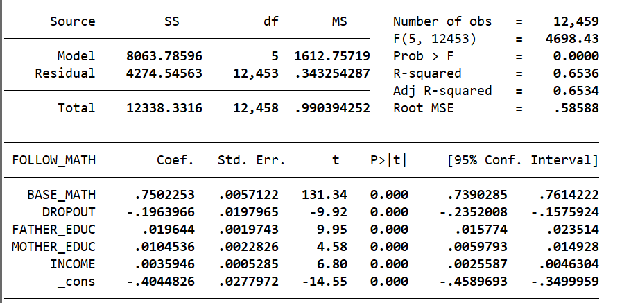
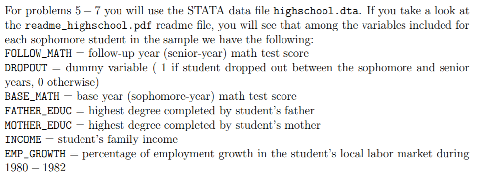
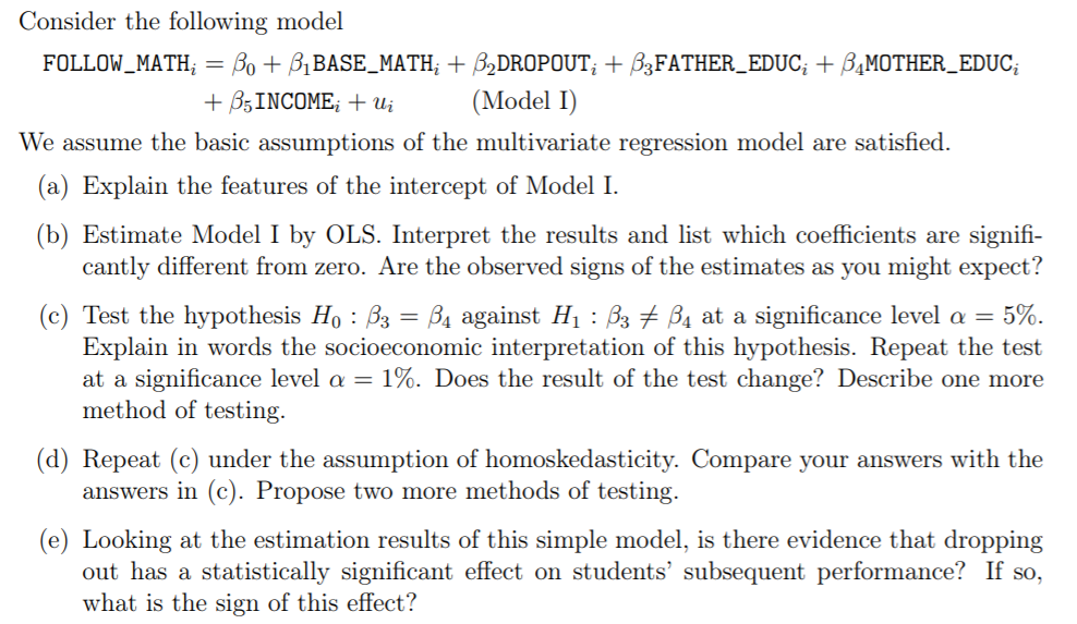
Source SS df MS Model Residual 8063.78596 4274.54563 5 1612.75719 12,453 .343254287 Number of obs F(5, 12453) Prob > F R-squared Adj R-squared Root MSE 12,459 4698.43 0.0000 0.6536 0.6534 .58588 Total 12338.3316 12,458 .990394252 FOLLOW_MATH Coef. Std. Err. t P>t. [95% Conf. Interval] BASE_MATH DROPOUT FATHER_EDUC MOTHER_EDUC INCOME _cons .7502253 -. 1963966 .019644 .0104536 .0035946 -.4044826 .0057122 .0197965 .0019743 .0022826 .0005285 .0277972 131.34 -9.92 9.95 4.58 6.80 -14.55 0.000 0.000 0.000 0.000 0.000 0.000 .7390285 -.2352008 .015774 .0059793 .0025587 -.4589693 .7614222 - . 1575924 .023514 .014928 .0046304 -.3499959 For problems 5 7 you will use the STATA data file highschool.dta. If you take a look at the readme_highschool.pdf readme file, you will see that among the variables included for each sophomore student in the sample we have the following: FOLLOW_MATH = follow-up year (senior-year) math test score DROPOUT = dummy variable ( 1 if student dropped out between the sophomore and senior years, 0 otherwise) BASE_MATH = base year (sophomore-year) math test score FATHER_EDUC highest degree completed by student's father MOTHER_EDUC = highest degree completed by student's mother INCOME = student's family income EMP_GROWTH = percentage of employment growth in the student's local labor market during 1980 - 1982 Consider the following model FOLLOW_MATH; = Bo + B1BASE_MATH; + B2DROPOUT; + B3FATHER_EDUC; + BAMOTHER_EDUC; + B5INCOME; + U (Model I) We assume the basic assumptions of the multivariate regression model are satisfied. (a) Explain the features of the intercept of Model I. (b) Estimate Model I by OLS. Interpret the results and list which coefficients are signifi- cantly different from zero. Are the observed signs of the estimates as you might expect? (c) Test the hypothesis Ho : B3 = B4 against Hp : 33 34 at a significance level a = 5%. Explain in words the socioeconomic interpretation of this hypothesis. Repeat the test at a significance level a = 1%. Does the result of the test change? Describe one more method of testing. (d) Repeat (C) under the assumption of homoskedasticity. Compare your answers with the answers in (c). Propose two more methods of testing. (e) Looking at the estimation results of this simple model, is there evidence that dropping out has a statistically significant effect on students' subsequent performance? If so, what is the sign of this effect? . Source SS df MS Model Residual 8063.78596 4274.54563 5 1612.75719 12,453 .343254287 Number of obs F(5, 12453) Prob > F R-squared Adj R-squared Root MSE 12,459 4698.43 0.0000 0.6536 0.6534 .58588 Total 12338.3316 12,458 .990394252 FOLLOW_MATH Coef. Std. Err. t P>t. [95% Conf. Interval] BASE_MATH DROPOUT FATHER_EDUC MOTHER_EDUC INCOME _cons .7502253 -. 1963966 .019644 .0104536 .0035946 -.4044826 .0057122 .0197965 .0019743 .0022826 .0005285 .0277972 131.34 -9.92 9.95 4.58 6.80 -14.55 0.000 0.000 0.000 0.000 0.000 0.000 .7390285 -.2352008 .015774 .0059793 .0025587 -.4589693 .7614222 - . 1575924 .023514 .014928 .0046304 -.3499959 For problems 5 7 you will use the STATA data file highschool.dta. If you take a look at the readme_highschool.pdf readme file, you will see that among the variables included for each sophomore student in the sample we have the following: FOLLOW_MATH = follow-up year (senior-year) math test score DROPOUT = dummy variable ( 1 if student dropped out between the sophomore and senior years, 0 otherwise) BASE_MATH = base year (sophomore-year) math test score FATHER_EDUC highest degree completed by student's father MOTHER_EDUC = highest degree completed by student's mother INCOME = student's family income EMP_GROWTH = percentage of employment growth in the student's local labor market during 1980 - 1982 Consider the following model FOLLOW_MATH; = Bo + B1BASE_MATH; + B2DROPOUT; + B3FATHER_EDUC; + BAMOTHER_EDUC; + B5INCOME; + U (Model I) We assume the basic assumptions of the multivariate regression model are satisfied. (a) Explain the features of the intercept of Model I. (b) Estimate Model I by OLS. Interpret the results and list which coefficients are signifi- cantly different from zero. Are the observed signs of the estimates as you might expect? (c) Test the hypothesis Ho : B3 = B4 against Hp : 33 34 at a significance level a = 5%. Explain in words the socioeconomic interpretation of this hypothesis. Repeat the test at a significance level a = 1%. Does the result of the test change? Describe one more method of testing. (d) Repeat (C) under the assumption of homoskedasticity. Compare your answers with the answers in (c). Propose two more methods of testing. (e) Looking at the estimation results of this simple model, is there evidence that dropping out has a statistically significant effect on students' subsequent performance? If so, what is the sign of this effect