**Please also shows the Excel Formula**

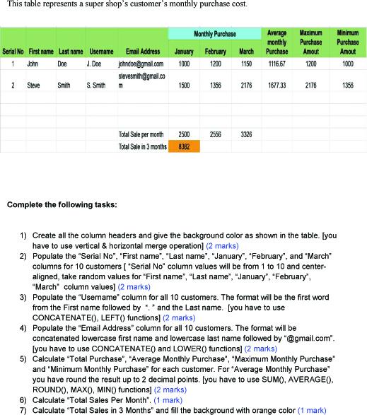
This table represents a super shop's customer's monthly purchase cost. Complete the following tasks: 1) Create all the column headers and give the background color as shown in the table. [you have to use vertical \& horizontal merge operation] ( 2 marks) 2) Populate the "Serial No", "First name", "Last name", "January", "February", and "March" columns for 10 customers [ "Serial No" column values will be from 1 to 10 and centeraligned, take random values for "First name", "Last name", "January", "February", "March" column values] ( 2 marks) 3) Populate the "Usemame" column for all 10 customers. The format will be the first word from the First name followed by ": " and the Last name. [you have to use CONCATENATE(), LEFT() functions] (2 marks) 4) Populate the "Email Address" column for all 10 customers. The format will be concatenated lowercase first name and lowercase last name followed by "@gmail.com". [you have to use CONCATENATE() and LOWER() functions] (2 marks) 5) Calculate "Total Purchase", "Average Monthly Purchase", "Maximum Monthly Purchase" and "Minimum Monthly Purchase" for each customer. For "Average Monthly Purchase" you have round the result up to 2 decimal points. [you have to use SUMO, AVERAGE(), ROUND0, MAX(), MINO functions] (2 marks) 6) Calculate "Total Sales Per Month". (1 mark) 7) Calculate "Total Sales in 3 Months" and fill the backaround with orange color (1 mark)