please answer instructions 1-9 for a like! please and thank you!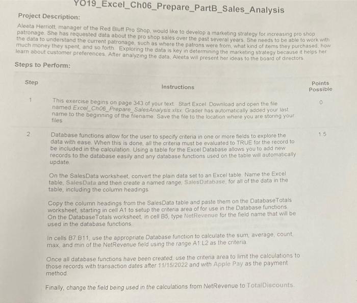

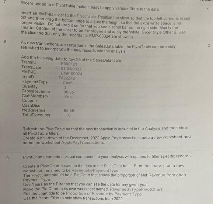
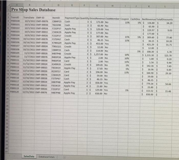
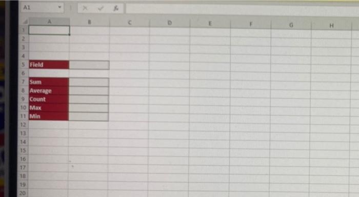
Y019_Excel_Ch06_Prepare_PartB_Sales_Analysis Project Description: Aleeta Herriott manager of the Red Blut Pro Shop, would like to develop a marketing strategy for increasing pro shop patronage. She has requested data about the pro shop sales over the past several years. She needs to be able to work with the data to understand the current patronage, such as where the patrons were from what kind of items they purchased how much money they spent, and so forth Exploring the data is key in determining the marketing strategy because it helps her learn about customer preferences. After analyzing the data. Aleeta will present her ideas to the board of directors Steps to Perform: Step Instructions Points Possible 1 0 This exercise begins on page 343 of your text Start Excel Download and open the file named Excel_Cho6_Prepare_SalesAnalysis xlsx Grader has automatically added your last name to the beginning of the filename Save the file to the location where you are storing your files 2 1.5 Database functions allow for the user to specify criteria in one or more fields to explore the data with ease When this is done, all the criters must be evaluated to TRUE for the record to be included in the calculation Using a table for the Excel Database allows you to add new records to the database easily and any database functions used on the table will automatically update On the Sales Data worksheet, convert the plain data set to an Excel table Name the Excel table, Sales Data and then create a named range, Sales Database for all of the data in the table, including the column headings Copy the column headings from the Sales Data table and paste them on the Database Totals worksheet, starting in cell A1 to setup the criteria area of for use in the Database functions On the Database Totals worksheet, in cell B5, type NetRevenue for the field name that will be used in the database functions In cells B7 B11, use the appropriate Database function to calculate the sum, average count max, and min of the NetRevenue field using the range A1 L2 as the criteria Once all database functions have been created, use the criteria area to limit the calculations to those records with transaction dates after 11/15/2022 and with Apple Pay as the payment method Finally, change the field being used in the calculations from NetRevenue to TotalDiscounts. Instructions 3 Excel's Recommended Pivot Tables feature allows you to easily explore data from many different perspectives with just a few clicks Once created, they can be easily modified to improve readability and even changed to further explore the data Points Possible 07 Using the data on the SalesData worksheet use the Recommended Pivot Table button on the Insert tab to create the Average of Cash Disc by Quantity Pivot Table If using a Mac the Recommended Pivot Table automatically created will need to be modified before moving forward In the PrvotTable Fields pane, click to deselect TransDate NetRevenue and EMP.D. In the Pivot Table Fields pane drag Quantity to Rows. Club Member? to columnis, and CashDisc to Values Right-click the Cash Disc field in the Values area, select Field Settings, and change the Summarize by function to Average Configure the Pivot Table Options so that error values are shown as 0 In cell A4 replace Row Labels with Quantity Sold an in cell 83, replace Column Labels with Cash Discount? Remove the CashDisc field from the Values area and replace it with the TotalDiscounts field Rename the worksheet to be TotalDiscounts Byty 4 13 A Pivot Table is an interactive table that extracts organizes and summarzes source data Pivot Tables are used for data analysis and looking for trends and patterns for decision- making purposes The first step in creating a Pivot Table is to select the data to be used and the location where it is to be created Use the data in the SalesData Excel Table to create a Pivot Table on a new worksheet Name the new worksheet PivotAnalysis 5 1.5 Seeing how the Net Revenue breaks down into various groups can be easily done with Pivot Tables Create a Pivottable that displays the NetRevenue values with the TransDate field grouped Into Years, Quarters and Months as the Rows and the Payment Type as the columns Use the Club Member? field as the report fiter and only show the data for club members 6 1 Pivot Tables can be made more user-friendly and provide additional insights into your data though various Pivot Table configuration options Create a Total Net Revenue Custom Name for the Sum of NetRevenue field and format the field as Accounting with 2 decimal place In cell A4, replace Row Labels with Quarters by Year and in cell B3, replace Column Labels with Payment Type Change the Pivot Table so that it shows the Total Net Revenue as % of Grand Total Apply the White Pivot Style Light 23 to the Pivot Table 2 Slicers added to a Pivottable make it easy to apply various filters to the data Insert an EMP-D slicer to the Pivot Table Position the slicer so that the top-left corner is in cell G3 and then drag the bottom edge to adjust the height so that the extra white space is no longer visible. Do not drag it so far that you see a scroll bar on the right side Modity the Header Caption of the slicer to be Employee and apply the White, Slicer Style Other 2. Uso the slicer so that only the records for EMP-00024 are showing As new transactions are recorded in the Sales Data table, the Pivottable can be easily refreshed to incorporate the new records into the analysis Add the following data to row 25 of the Sales Data table Transit P000121 TransDate 01/01/2023 EMP-ID EMP-00024 Itemid T822248 Payment Type Cash Quantity GrossRevenue 98.85 Club Member? Yes Coupon Cash Disc NetRevenue 98.85 TotalDiscounts 3 0 Refresh the PivotTable so that the new transaction is included in the Analysis and then clear all Pivot Table filters Create a drill-down of the December, 2022 Apple Pay transactions onto a new worksheet and name the worksheet ApplePayTransactions. 9 PivotCharts can add a visual component to your analysis with options to filter specific records Create a PivotChart based on the data in the Sales Data table Start the analysis on a new worksheet, renamed to be RevenueByPaymentType The PivotChart should be a Pie Chart that shows the proportion of Net Revenue from each Payment Type Use Years as the filter so that you can see the data for any given year Move the Pie Chart to its own worksheet named, RevenueByTypePivotChart Edit the chart title to be proportion of Revenue by Payment Type Use the Years Filter to only show transactions from 2022 G K Pro Shop Sales Database 2 3 TransID 4 P000100 5 P000101 PO00102 7 PO00103 8 PO00104 9 P000105 10 P00106 11 P000107 12 PO00108 13 P000109 14 PO00110 15 P000111 16 P000112 17 PO00113 1 PO00114 19 P000115 20 PO00116 21 P00117 22 PO00118 23 PO00119 24 PO00120 25 26 27 28 29 30 31 32 33 34 35 36 37 38 39 TransDate EMP-ID 10/3/2022 EMP-00076 10/3/2002 EMP-00038 10/3/2032 EMP-00024 10/5/2022 EMP-00025 10/6/2022 EMP-00026 10/12/2022 EMP-00025 10/16/2022 EMP-00038 10/22/2022 EMP-00024 10/25/2022 EMP-COOLS 11/2/2022 EMP-00026 11/7/2022 EMP-00075 11/10/2022 EMP-00038 11/13/2022 EMP-00024 11/21/2022 EMP-0015 12/13/2022 EMP-00036 12/14/2022 EMP-00026 12/16/2022 EMP-00038 12/10/2022 EMP-00034 12/24/2022 EMP-00015 12/29/2022 EMP-00026 12/31/2022 EMP-00076 Itemid PaymentTyp Quantity GrossRevenue Club Member Coupon Cash Disc NetRevenue TotalDiscounts CSP 23 Cash 3 S 171.00 No 15% 5% $ 136.80 $ 34.20 T802248 Cash 2. $ 65.90 No $ 65.90$ F232237 Apple Pay 1$ 129.00 Yes S 119.97 S 9.03 CSB3K28 Apple Pay 3 S 177.00 No $ 177.00 $ F232P37 Credit 3 S 387.00 No 15% 5% $ 309.60 $ 77.40 F375PS Cash 3 $ 46.35 Yes 15% $ 36.15 S 10.20 X140029 Apple Pay 1 S 453.00 Yes S 421.29 $ 31.71 T981011 Credit 1$ 12.00 NO $ 12.00 S CSS4P23 Cash 2 S 114.00 No 5% S 108.30 $ 5.70 XAT Credit 3 $ 1,257.00 NO 10% $ 1,131.30$ 125.20 RAR3P24 Apple Pay 18 2.00 NO 10% S 1.80 $ 0.20 RAROP24 Card 1 $ 2.00 Yes 1.56 $ 0.14 X34939 Credit 3 S 149.85 NO 5% $ 142.36 $ 7.49 783319 Apple Pay 3 $ 17.85 NO 5% S 16.96S 0.89 R29157 Card 2 $ 14.00 No 15% S 164.90 S 29.10 CSS329 Card 1 S 59.00 No S 59.00 $ F375P67 Cash 3 $ 46.15 No S 46.35 S XAS Apple Pay 2 S 838.00 Yes $ 779.345 58.66 F3319 Apple Pay 4 S 23.80 No $ 23.80 $ F232P37 Card 1 $ 129.00 Yes 5% $ 113.52 S 15.48 X48748 Apple Pay 2. $ 838.00 No 838.00 $ 25% 40 41 Sales Data Database Totals H 2 3 4 5 Field 6 7 Sum 8 Average 9 Count 10 Max 11 Min 12 13 14 15 16 17 18 19 20 Y019_Excel_Ch06_Prepare_PartB_Sales_Analysis Project Description: Aleeta Herriott manager of the Red Blut Pro Shop, would like to develop a marketing strategy for increasing pro shop patronage. She has requested data about the pro shop sales over the past several years. She needs to be able to work with the data to understand the current patronage, such as where the patrons were from what kind of items they purchased how much money they spent, and so forth Exploring the data is key in determining the marketing strategy because it helps her learn about customer preferences. After analyzing the data. Aleeta will present her ideas to the board of directors Steps to Perform: Step Instructions Points Possible 1 0 This exercise begins on page 343 of your text Start Excel Download and open the file named Excel_Cho6_Prepare_SalesAnalysis xlsx Grader has automatically added your last name to the beginning of the filename Save the file to the location where you are storing your files 2 1.5 Database functions allow for the user to specify criteria in one or more fields to explore the data with ease When this is done, all the criters must be evaluated to TRUE for the record to be included in the calculation Using a table for the Excel Database allows you to add new records to the database easily and any database functions used on the table will automatically update On the Sales Data worksheet, convert the plain data set to an Excel table Name the Excel table, Sales Data and then create a named range, Sales Database for all of the data in the table, including the column headings Copy the column headings from the Sales Data table and paste them on the Database Totals worksheet, starting in cell A1 to setup the criteria area of for use in the Database functions On the Database Totals worksheet, in cell B5, type NetRevenue for the field name that will be used in the database functions In cells B7 B11, use the appropriate Database function to calculate the sum, average count max, and min of the NetRevenue field using the range A1 L2 as the criteria Once all database functions have been created, use the criteria area to limit the calculations to those records with transaction dates after 11/15/2022 and with Apple Pay as the payment method Finally, change the field being used in the calculations from NetRevenue to TotalDiscounts. Instructions 3 Excel's Recommended Pivot Tables feature allows you to easily explore data from many different perspectives with just a few clicks Once created, they can be easily modified to improve readability and even changed to further explore the data Points Possible 07 Using the data on the SalesData worksheet use the Recommended Pivot Table button on the Insert tab to create the Average of Cash Disc by Quantity Pivot Table If using a Mac the Recommended Pivot Table automatically created will need to be modified before moving forward In the PrvotTable Fields pane, click to deselect TransDate NetRevenue and EMP.D. In the Pivot Table Fields pane drag Quantity to Rows. Club Member? to columnis, and CashDisc to Values Right-click the Cash Disc field in the Values area, select Field Settings, and change the Summarize by function to Average Configure the Pivot Table Options so that error values are shown as 0 In cell A4 replace Row Labels with Quantity Sold an in cell 83, replace Column Labels with Cash Discount? Remove the CashDisc field from the Values area and replace it with the TotalDiscounts field Rename the worksheet to be TotalDiscounts Byty 4 13 A Pivot Table is an interactive table that extracts organizes and summarzes source data Pivot Tables are used for data analysis and looking for trends and patterns for decision- making purposes The first step in creating a Pivot Table is to select the data to be used and the location where it is to be created Use the data in the SalesData Excel Table to create a Pivot Table on a new worksheet Name the new worksheet PivotAnalysis 5 1.5 Seeing how the Net Revenue breaks down into various groups can be easily done with Pivot Tables Create a Pivottable that displays the NetRevenue values with the TransDate field grouped Into Years, Quarters and Months as the Rows and the Payment Type as the columns Use the Club Member? field as the report fiter and only show the data for club members 6 1 Pivot Tables can be made more user-friendly and provide additional insights into your data though various Pivot Table configuration options Create a Total Net Revenue Custom Name for the Sum of NetRevenue field and format the field as Accounting with 2 decimal place In cell A4, replace Row Labels with Quarters by Year and in cell B3, replace Column Labels with Payment Type Change the Pivot Table so that it shows the Total Net Revenue as % of Grand Total Apply the White Pivot Style Light 23 to the Pivot Table 2 Slicers added to a Pivottable make it easy to apply various filters to the data Insert an EMP-D slicer to the Pivot Table Position the slicer so that the top-left corner is in cell G3 and then drag the bottom edge to adjust the height so that the extra white space is no longer visible. Do not drag it so far that you see a scroll bar on the right side Modity the Header Caption of the slicer to be Employee and apply the White, Slicer Style Other 2. Uso the slicer so that only the records for EMP-00024 are showing As new transactions are recorded in the Sales Data table, the Pivottable can be easily refreshed to incorporate the new records into the analysis Add the following data to row 25 of the Sales Data table Transit P000121 TransDate 01/01/2023 EMP-ID EMP-00024 Itemid T822248 Payment Type Cash Quantity GrossRevenue 98.85 Club Member? Yes Coupon Cash Disc NetRevenue 98.85 TotalDiscounts 3 0 Refresh the PivotTable so that the new transaction is included in the Analysis and then clear all Pivot Table filters Create a drill-down of the December, 2022 Apple Pay transactions onto a new worksheet and name the worksheet ApplePayTransactions. 9 PivotCharts can add a visual component to your analysis with options to filter specific records Create a PivotChart based on the data in the Sales Data table Start the analysis on a new worksheet, renamed to be RevenueByPaymentType The PivotChart should be a Pie Chart that shows the proportion of Net Revenue from each Payment Type Use Years as the filter so that you can see the data for any given year Move the Pie Chart to its own worksheet named, RevenueByTypePivotChart Edit the chart title to be proportion of Revenue by Payment Type Use the Years Filter to only show transactions from 2022 G K Pro Shop Sales Database 2 3 TransID 4 P000100 5 P000101 PO00102 7 PO00103 8 PO00104 9 P000105 10 P00106 11 P000107 12 PO00108 13 P000109 14 PO00110 15 P000111 16 P000112 17 PO00113 1 PO00114 19 P000115 20 PO00116 21 P00117 22 PO00118 23 PO00119 24 PO00120 25 26 27 28 29 30 31 32 33 34 35 36 37 38 39 TransDate EMP-ID 10/3/2022 EMP-00076 10/3/2002 EMP-00038 10/3/2032 EMP-00024 10/5/2022 EMP-00025 10/6/2022 EMP-00026 10/12/2022 EMP-00025 10/16/2022 EMP-00038 10/22/2022 EMP-00024 10/25/2022 EMP-COOLS 11/2/2022 EMP-00026 11/7/2022 EMP-00075 11/10/2022 EMP-00038 11/13/2022 EMP-00024 11/21/2022 EMP-0015 12/13/2022 EMP-00036 12/14/2022 EMP-00026 12/16/2022 EMP-00038 12/10/2022 EMP-00034 12/24/2022 EMP-00015 12/29/2022 EMP-00026 12/31/2022 EMP-00076 Itemid PaymentTyp Quantity GrossRevenue Club Member Coupon Cash Disc NetRevenue TotalDiscounts CSP 23 Cash 3 S 171.00 No 15% 5% $ 136.80 $ 34.20 T802248 Cash 2. $ 65.90 No $ 65.90$ F232237 Apple Pay 1$ 129.00 Yes S 119.97 S 9.03 CSB3K28 Apple Pay 3 S 177.00 No $ 177.00 $ F232P37 Credit 3 S 387.00 No 15% 5% $ 309.60 $ 77.40 F375PS Cash 3 $ 46.35 Yes 15% $ 36.15 S 10.20 X140029 Apple Pay 1 S 453.00 Yes S 421.29 $ 31.71 T981011 Credit 1$ 12.00 NO $ 12.00 S CSS4P23 Cash 2 S 114.00 No 5% S 108.30 $ 5.70 XAT Credit 3 $ 1,257.00 NO 10% $ 1,131.30$ 125.20 RAR3P24 Apple Pay 18 2.00 NO 10% S 1.80 $ 0.20 RAROP24 Card 1 $ 2.00 Yes 1.56 $ 0.14 X34939 Credit 3 S 149.85 NO 5% $ 142.36 $ 7.49 783319 Apple Pay 3 $ 17.85 NO 5% S 16.96S 0.89 R29157 Card 2 $ 14.00 No 15% S 164.90 S 29.10 CSS329 Card 1 S 59.00 No S 59.00 $ F375P67 Cash 3 $ 46.15 No S 46.35 S XAS Apple Pay 2 S 838.00 Yes $ 779.345 58.66 F3319 Apple Pay 4 S 23.80 No $ 23.80 $ F232P37 Card 1 $ 129.00 Yes 5% $ 113.52 S 15.48 X48748 Apple Pay 2. $ 838.00 No 838.00 $ 25% 40 41 Sales Data Database Totals H 2 3 4 5 Field 6 7 Sum 8 Average 9 Count 10 Max 11 Min 12 13 14 15 16 17 18 19 20