Please answer questions 2, 3 , 3 based on the text above .

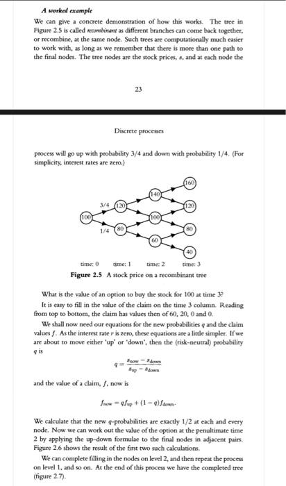
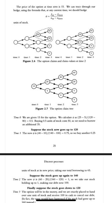
A worked example We can give a concrete demonstration of how this works. The tree in Figure 25 is called recombinant as different branches can come back together. of recombine, at the same node. Such trees are computationally much easier to work with, as long as we remember that there is more than one path to the final nodes. The tree nodes are the stock prices, s, and at each node the 23 Discrete processes process will go up with probability 3/4 and down with probability 1/4. (For simplicity, interest rates are zero.) 160 140 3/4 120 100 80 1/4 40 time: 0 time: 1 time: 2 time: 3 Figure 2.5 Astock price on a recombinant tree What is the value of an option to buy the stock for 100 at time 3? It is easy to fill in the value of the claim on the time 3 column. Reading from top to bottom, the claim has values then of 60, 20,0 and O. We shall now need our equations for the new probabilities and the claim values. As the interest rater is zero, these equations are a little simpler. If we are about to move either 'up' or 'down", then the (risk-neutral) probability qis Bowdown Bup-down and the value of a claim, /. now is w = 98 + (1 - San We calculate that the new g-probabilities are exactly 1/2 at each and every node. Now we can work out the value of the option at the penultimate time 2 by applying the up-down formulae to the final nodes in adjacent pairs. Figure 2.6 shows the result of the first two such calculations. We can complete filling in the nodes on level 2, and then repeat the process on level 1. and so on. At the end of this process we have the completed tree (figure 2.7). The price of the option at time zero is 15. We can trace through our hedge, using the formula that, at any current time, we should hedge - Sup-down units of stock time: 0 time: 3 time: 1 time: 0 time: 1 time: 2 Figure 2.6 The option claims and daim-values at time 2 time: 2 time: 3 time: 0 Figure 2.7 The option claim tree Time 0 We are given 15 for the option. We calculate oas (25 - 5)/(120 - 80) = 0.5. Buying 0.5 units of stock costs 50, so we need to borrow an additional 35. Suppose the stock now goes up to 120 Time 1 The new ois (40 - 10)/(140 - 100) = 0.75, so we buy another 0.25 25 Discrete processes units of stock at its new price, taking our total borrowing to 65. Suppose the stock goes up again to 140 Time 2 The new ois (60 - 20)/(160 - 120) - 1. so we take our stock holding up to 1, making our debt now 100. Finally suppose the stock goes down to 120 Time 3 The option will be in the money, and we are exactly placed to hand over one unit of stock and receive 100 in cash to cancel our debt. (In fact, the game where the stock had gone up to 10 instad) 2. Page 23. We use a recombinant tree, so that the number of paths to the final node is not always one. Figure 2.5 p 24 describes the stock price process. The probabilities are, as in the book, up and down. What is the value of an option, with strike price 90, at time 3. Produce the claim tree corresponding to Figure 2.7. With a strike price 90 the claim values are not as given in the book. 3. Produce the hedging results corresponding to Tables 2.3, 2.2, and one other path. A worked example We can give a concrete demonstration of how this works. The tree in Figure 25 is called recombinant as different branches can come back together. of recombine, at the same node. Such trees are computationally much easier to work with, as long as we remember that there is more than one path to the final nodes. The tree nodes are the stock prices, s, and at each node the 23 Discrete processes process will go up with probability 3/4 and down with probability 1/4. (For simplicity, interest rates are zero.) 160 140 3/4 120 100 80 1/4 40 time: 0 time: 1 time: 2 time: 3 Figure 2.5 Astock price on a recombinant tree What is the value of an option to buy the stock for 100 at time 3? It is easy to fill in the value of the claim on the time 3 column. Reading from top to bottom, the claim has values then of 60, 20,0 and O. We shall now need our equations for the new probabilities and the claim values. As the interest rater is zero, these equations are a little simpler. If we are about to move either 'up' or 'down", then the (risk-neutral) probability qis Bowdown Bup-down and the value of a claim, /. now is w = 98 + (1 - San We calculate that the new g-probabilities are exactly 1/2 at each and every node. Now we can work out the value of the option at the penultimate time 2 by applying the up-down formulae to the final nodes in adjacent pairs. Figure 2.6 shows the result of the first two such calculations. We can complete filling in the nodes on level 2, and then repeat the process on level 1. and so on. At the end of this process we have the completed tree (figure 2.7). The price of the option at time zero is 15. We can trace through our hedge, using the formula that, at any current time, we should hedge - Sup-down units of stock time: 0 time: 3 time: 1 time: 0 time: 1 time: 2 Figure 2.6 The option claims and daim-values at time 2 time: 2 time: 3 time: 0 Figure 2.7 The option claim tree Time 0 We are given 15 for the option. We calculate oas (25 - 5)/(120 - 80) = 0.5. Buying 0.5 units of stock costs 50, so we need to borrow an additional 35. Suppose the stock now goes up to 120 Time 1 The new ois (40 - 10)/(140 - 100) = 0.75, so we buy another 0.25 25 Discrete processes units of stock at its new price, taking our total borrowing to 65. Suppose the stock goes up again to 140 Time 2 The new ois (60 - 20)/(160 - 120) - 1. so we take our stock holding up to 1, making our debt now 100. Finally suppose the stock goes down to 120 Time 3 The option will be in the money, and we are exactly placed to hand over one unit of stock and receive 100 in cash to cancel our debt. (In fact, the game where the stock had gone up to 10 instad) 2. Page 23. We use a recombinant tree, so that the number of paths to the final node is not always one. Figure 2.5 p 24 describes the stock price process. The probabilities are, as in the book, up and down. What is the value of an option, with strike price 90, at time 3. Produce the claim tree corresponding to Figure 2.7. With a strike price 90 the claim values are not as given in the book. 3. Produce the hedging results corresponding to Tables 2.3, 2.2, and one other path