Please complete Section 3 in MATLAB

Please do not copy the answer from the previous chegg posts

Some useful information for this task can be found below:

(write the code assuming that you have all the necessary files for Section 3)

The template code can be seen below (please complete Section 3. Other sections are not necessary):

%% Main Body -- Do NOT edit

if ~exist('suppress_figures','var')

clc; clear; close all;

show_plots = 1;

else

show_plots = 0;

end

%% %%%%%%%%%%%%%%%%%%%%%%%%%%%%%%%%%%%%%%%%%%%%%%%%%%%%%%%

%%%%%%%%%%%%%% Section 1 %%%%%%%%%%%%%%

%%%%%%%%%%%%%% PERCEPTRON %%%%%%%%%%%%%%

%%%%%%%%%%%%%%%%%%%%%%%%%%%%%%%%%%%%%%%%%%%%%%%%%%%%%%%%%%

load('data_xor'); % data set in the shape of XOR, loads: X_tr X_te t_tr t_te

I = 400; % number of training iterations

gamma = 0.2; % learning rate

thetaA = [-0.1;1.2];

thetaB = [-0.1;1.2;0.9];

% Function 1

t_hatA= perceptron_predict( UA(X_tr), thetaA );

t_hatB= perceptron_predict( UB(X_tr), thetaB );

% Function 2

grad_thetaA = perceptron_gradient( UA(X_tr(17,:)).', t_tr(17), thetaA );

grad_thetaB = perceptron_gradient( UB(X_tr(17,:)).', t_tr(17), thetaB );

% Function 3

loss_per_de_A = detection_error_loss( UA(X_te), t_te, thetaA );

loss_per_de_B = detection_error_loss( UB(X_te), t_te, thetaB );

% Function 4

loss_per_A = hinge_at_zero_loss( UA(X_te), t_te, thetaA );

loss_per_B = hinge_at_zero_loss( UB(X_te), t_te, thetaB );

% Function 5

theta_per_matA = perceptron_train_sgd( UA(X_tr), t_tr, thetaA, I, gamma );

theta_per_matB = perceptron_train_sgd( UB(X_tr), t_tr, thetaB, I, gamma );

if show_plots % perceprton

vec_loss_per_hoz_teA = zeros(1,I+1);

vec_loss_per_hoz_teB = zeros(1,I+1);

vec_loss_per_de_teA = zeros(1,I+1);

vec_loss_per_de_teB = zeros(1,I+1);

for ii=1:(I+1)

vec_loss_per_hoz_teA(ii) = hinge_at_zero_loss( UA(X_te), t_te, theta_per_matA(:,ii) );

vec_loss_per_hoz_teB(ii) = hinge_at_zero_loss( UB(X_te), t_te, theta_per_matB(:,ii) );

vec_loss_per_de_teA(ii) = detection_error_loss( UA(X_te), t_te, theta_per_matA(:,ii) );

vec_loss_per_de_teB(ii) = detection_error_loss( UB(X_te), t_te, theta_per_matB(:,ii) );

end

figure;

plot(0:I,vec_loss_per_hoz_teA,'mo--' ,'DisplayName','features A; hinge-at-zero loss'); hold on;

plot(0:I,vec_loss_per_hoz_teB,'go--' ,'DisplayName','features B; hinge-at-zero loss');

plot(0:I,vec_loss_per_de_teA ,'m-','DisplayName','features A; detection-error loss'); hold on;

plot(0:I,vec_loss_per_de_teB ,'g-','DisplayName','features B; detection-error loss');

xlabel('Iteration','interpreter','latex');

ylabel('loss','interpreter','latex');

title ('Perceptron test losses','interpreter','latex');

legend show; grid;

figure;

plot_perceptron(theta_per_matA,X_te,t_te,@UA,'Perceptron: original features');

figure;

plot_perceptron(theta_per_matB,X_te,t_te,@UB,'Perceptron: extended features');

legend show;

end

% Function 6

discussionA();

%% %%%%%%%%%%%%%%%%%%%%%%%%%%%%%%%%%%%%%%%%%%%%%%%%%%%%%%%

%%%%%%%%%%%%%% Section 2 %%%%%%%%%%%%%%

%%%%%%%%%%%%%% LOGISTIC REGRESSION %%%%%%%%%%%%%%

%%%%%%%%%%%%%%%%%%%%%%%%%%%%%%%%%%%%%%%%%%%%%%%%%%%%%%%%%%

S = 30; % mini-batch size

thetaA = [-0.1;1.2];

thetaB = [-0.1;1.2;0.9];

% Function 7

logit_hatA= logistic_regression_logit( UA(X_tr), thetaA );

logit_hatB= logistic_regression_logit( UB(X_tr), thetaB );

% Function 8

grad_thetaA = logistic_regression_gradient( UA(X_tr(17,:)).', t_tr(17), thetaA );

grad_thetaB = logistic_regression_gradient( UB(X_tr(17,:)).', t_tr(17), thetaB );

% Function 9

loss_lr_A = logistic_loss( UA(X_te), t_te, thetaA );

loss_lr_B = logistic_loss( UB(X_te), t_te, thetaB );

% Function 10

theta_lr_matA = logistic_regression_train_sgd( UA(X_tr), t_tr, thetaA, I, gamma, S );

theta_lr_matB = logistic_regression_train_sgd( UB(X_tr), t_tr, thetaB, I, gamma, S );

% code for evalutating the test loss while training

vec_loss_lr_lo_teA = zeros(1,I+1);

vec_loss_lr_lo_teB = zeros(1,I+1);

vec_loss_lr_de_teA = zeros(1,I+1);

vec_loss_lr_de_teB = zeros(1,I+1);

for ii=1:(I+1)

vec_loss_lr_lo_teA(ii) = logistic_loss( UA(X_te), t_te, theta_lr_matA(:,ii) );

vec_loss_lr_lo_teB(ii) = logistic_loss( UB(X_te), t_te, theta_lr_matB(:,ii) );

vec_loss_lr_de_teA(ii) = detection_error_loss( UA(X_te), t_te, theta_lr_matA(:,ii) );

vec_loss_lr_de_teB(ii) = detection_error_loss( UB(X_te), t_te, theta_lr_matB(:,ii) );

end

% auxiliary code for plotting

if show_plots % logistic regression

figure;

plot(0:I,vec_loss_lr_lo_teA,'mo--','DisplayName','features A; logistic loss'); hold on;

plot(0:I,vec_loss_lr_lo_teB,'go--','DisplayName','features B; logistic loss');

plot(0:I,vec_loss_lr_de_teA,'m-','DisplayName','features A; detection-error loss'); hold on;

plot(0:I,vec_loss_lr_de_teB,'g-','DisplayName','features B; detection-error loss');

xlabel('Iteration','interpreter','latex');

ylabel('loss','interpreter','latex');

title ('Logistic Regression test loss','interpreter','latex');

legend show; grid;

figure;

plot_logistic_regression(theta_lr_matA,X_te,t_te,@UA,'Logistic Regression: original features');

figure;

plot_logistic_regression(theta_lr_matB,X_te,t_te,@UB,'Logistic Regression: extended features');

end

%% %%%%%%%%%%%%%%%%%%%%%%%%%%%%%%%%%%%%%%%%%%%%%%%%%%%%%%%

%%%%%%%%%%%%%% Section 3 %%%%%%%%%%%%%%

%%%%%%%%%%%%%% NEURAL NETWORKS %%%%%%%%%%%%%%

%%%%%%%%%%%%%%%%%%%%%%%%%%%%%%%%%%%%%%%%%%%%%%%%%%%%%%%%%%

theta_nn.W1 = [-0.1,+0.2;-0.5,-0.7;+0.4,+0.8];

theta_nn.W2 = [-0.6,+1.1,-0.9;+1.4,-0.6,-0.5];

theta_nn.w3 = [-0.2;+0.8];

x1_nn = [-1.0;-0.5];

t1_nn = 1;

x2_nn = [-0.4;+0.2];

t2_nn = 1;

% Function 11

[logit1_nn,record1] = neural_network_logit( x1_nn, theta_nn); % 'record1' is not graded, can be left empty

[logit2_nn,record2] = neural_network_logit( x2_nn, theta_nn); % 'record2' is not graded, can be left empty

% Function 12

grad_ReLU1_nn = grad_ReLU( x1_nn);

grad_ReLU2_nn = grad_ReLU( x2_nn);

% Function 13

grad1_theta_nn = neural_network_gradient( x1_nn, t1_nn, theta_nn);

grad2_theta_nn = neural_network_gradient( x2_nn, t2_nn, theta_nn);

%% %%%%%%%%%%%%%%%%%%%%%%%%%%%%%%%%%%%%%%%%%%%%%%%%%%%%%%%

%%%%%%%%%%%%%% Section 4 %%%%%%%%%%%%%%

%%%%%%%%%%%%%% PCA %%%%%%%%%%%%%%

%%%%%%%%%%%%%%%%%%%%%%%%%%%%%%%%%%%%%%%%%%%%%%%%%%%%%%%%%%

load dats_usps_5_6 X t;

if show_plots

figure; sgtitle('Random 24 samples of 5 and 6 digits from USPS data set');

for n=1:4*6

subplot(4,6,n);

show_vec_as_image16x16(X(n,:));

title(['t_{',num2str(n),'}=',num2str(t(n)),' x_{',num2str(n),'}=']);

end

end

mu_hat = mean(X,1); % empirical_average as a row vector

Xub = X - mu_hat ; % matrix minus row = row-wise subtraction

x = Xub(1,:).';

% Function 14

W3 = pca_get_dict(Xub,3);

W6 = pca_get_dict(Xub,6);

% Function 15

z3 = pca_encode(x,W3);

z6 = pca_encode(x,W6);

% Function 16

x_hat3 = pca_decode(z3,W3);

x_hat6 = pca_decode(z6,W6);

% auxiliary code for plotting

if show_plots

Nvec = [2,5,7,24,27];

Mvec = [0,1,3,30];

figure;

for nn=1:length(Nvec)

n = Nvec(nn);

x = Xub(n,:).';

for mm=1:length(Mvec)

M = Mvec(mm);

W = pca_get_dict(Xub,M);

z = pca_encode(x,W);

x_hat = pca_decode(z,W);

subplot(length(Mvec),length(Nvec),nn+(mm-1)*length(Nvec));

show_vec_as_image16x16(x_hat.' + mu_hat); % adding back the empirical mean

title(['n=',num2str(n),' M=',num2str(M),' t=',num2str(t(n))]);

end

end

end

% Function 17

discussionB();

%% %%%%%%%%%%%%%%%%%%%%%%%%%%%%%%%%%%%%%%%%%%%%%%%%%%%%%%%

%%%%%%%%%%%%%% AUXILIARY FUNCTIONS %%%%%%%%%%%%%%

%%%%%%%%%%%%%%%%%%%%%%%%%%%%%%%%%%%%%%%%%%%%%%%%%%%%%%%%%%

function U = UA(X)

U = X;

end

function U = UB(X)

U = [X , X(:,1) .* X(:,2) ];

end

function out = sigmoid(in)

out = 1./(1+exp(-in));

end

function plot_perceptron(theta_mat,X_te,t_te,U,title_str)

I = size(theta_mat,2)-1;

D = size(theta_mat,1);

Ngrid = 101; % number of ponts in grid

[mX1,mX2] = meshgrid(linspace(-1,1,Ngrid),linspace(-1,1,Ngrid));

X_gr = [mX1(:),mX2(:)]; % gr for grid

tiledlayout(2,2);

for ii=1:4

nexttile;

t_hat= perceptron_predict( U(X_gr), theta_mat(:,round(2.^(ii-4)*I)) );

contourf(mX1,mX2,max(0,min(1,reshape(t_hat,[Ngrid,Ngrid]))),'ShowText','on','DisplayName','LS solution'); inc_vec = linspace(0,1,11).'; colormap([inc_vec,1-inc_vec,0*inc_vec]); hold on;

plot(X_te(t_te==0,1),X_te(t_te==0,2),'o','MarkerSize',6,'MarkerEdgeColor','k','MarkerFaceColor','c','DisplayName','t=0 test');

plot(X_te(t_te==1,1),X_te(t_te==1,2),'^','MarkerSize',6,'MarkerEdgeColor','k','MarkerFaceColor','m','DisplayName','t=1 test');

contour (mX1,mX2,max(0,min(1,reshape(t_hat,[Ngrid,Ngrid]))),[0.5,0.5],'y--','LineWidth',3,'DisplayName','Decision line');

xlabel('$x_1$','interpreter','latex'); ylabel('$x_2$','interpreter','latex'); colorbar; title([title_str, ' iters=',num2str(round(2.^(ii-4)*I))],'interpreter','latex'); legend show;

end

end

function plot_logistic_regression(theta_mat,X_te,t_te,U,title_str)

I = size(theta_mat,2)-1;

D = size(theta_mat,1);

Ngrid = 51; % number of ponts in grid

[mX1,mX2] = meshgrid(linspace(-1,1,Ngrid),linspace(-1,1,Ngrid));

X_gr = [mX1(:),mX2(:)]; % gr for grid

tiledlayout(2,2);

for ii=1:4

nexttile;

logit= logistic_regression_logit( U(X_gr), theta_mat(:,round(2.^(ii-4)*I)) );

prob_t_1 = sigmoid(logit);

contourf(mX1,mX2,max(0,min(1,reshape(prob_t_1,[Ngrid,Ngrid]))),'ShowText','on','DisplayName','LS solution'); inc_vec = linspace(0,1,11).'; colormap([inc_vec,1-inc_vec,0*inc_vec]); hold on;

plot(X_te(t_te==0,1),X_te(t_te==0,2),'o','MarkerSize',6,'MarkerEdgeColor','k','MarkerFaceColor','c','DisplayName','t=0 test');

plot(X_te(t_te==1,1),X_te(t_te==1,2),'^','MarkerSize',6,'MarkerEdgeColor','k','MarkerFaceColor','m','DisplayName','t=1 test');

contour (mX1,mX2,max(0,min(1,reshape(prob_t_1,[Ngrid,Ngrid]))),[0.5,0.5],'y--','LineWidth',3,'DisplayName','Decision line');

xlabel('$x_1$','interpreter','latex'); ylabel('$x_2$','interpreter','latex'); colorbar; title([title_str, ' iters=',num2str(round(2.^(ii-4)*I))],'interpreter','latex'); legend show;

end

end

function out = ReLU(in)

out = in.*(in > 0);

end

function out = show_vec_as_image16x16(row_vec)

out = imshow(-(reshape(row_vec,16,16)).'); % shows the image of a row vector with 256 elements. For matching purposes, a negation and rotation are needed.

end

%%%%%%%%%%%%%%%%%%%%%%%%%%%%%%%%%%%%%%%%%%%%%%%%%%%%%%%%%%

%%%%%% INSERT YOUR CODE IN THE FUNCTIONS BELOW %%%%%%%%

%%%%%%%%%%%%%%%%%%%%%%%%%%%%%%%%%%%%%%%%%%%%%%%%%%%%%%%%%%

% Function 11

function [logit,record] = neural_network_logit(x, theta)

logit = rand(1);

record = []; % if you do not use record, leave this line to prevent errors

% DELETE ABOVE 2 LINES AND THIS COMMENT, AND PLACE YOUR CODE INSTEAD

end

% Function 12

function out = grad_ReLU(in)

out = in;

% DELETE ABOVE LINE AND THIS COMMENT, AND PLACE YOUR CODE INSTEAD

end

% Function 13

function grad_theta = neural_network_gradient(x,t,theta)

grad_theta.w3 = randn(size(theta.w3));

grad_theta.W2 = randn(size(theta.W2));

grad_theta.W1 = randn(size(theta.W1));

% DELETE ABOVE 3 LINES AND THIS COMMENT, AND PLACE YOUR CODE INSTEAD

end

Important remarks:

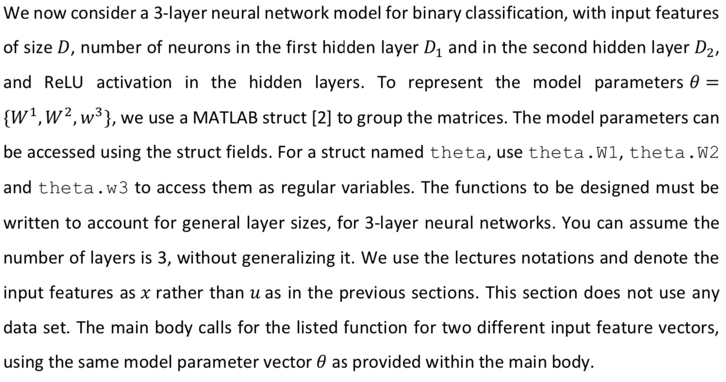
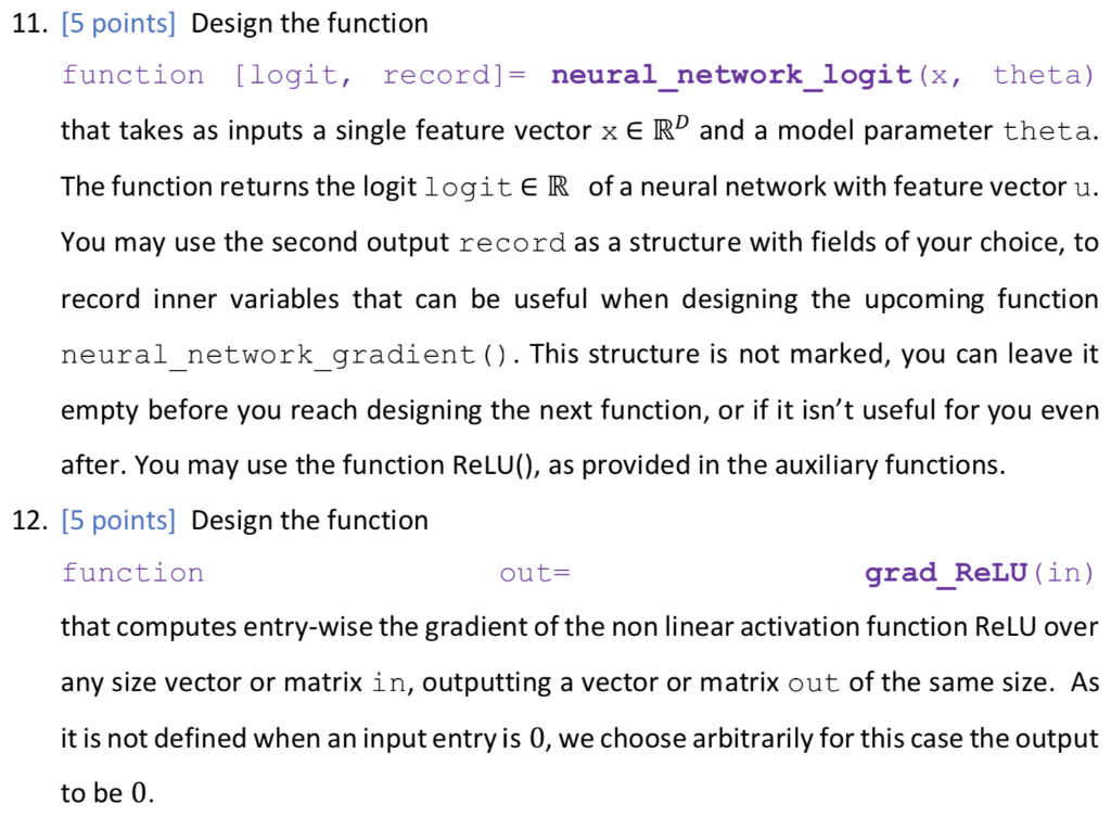
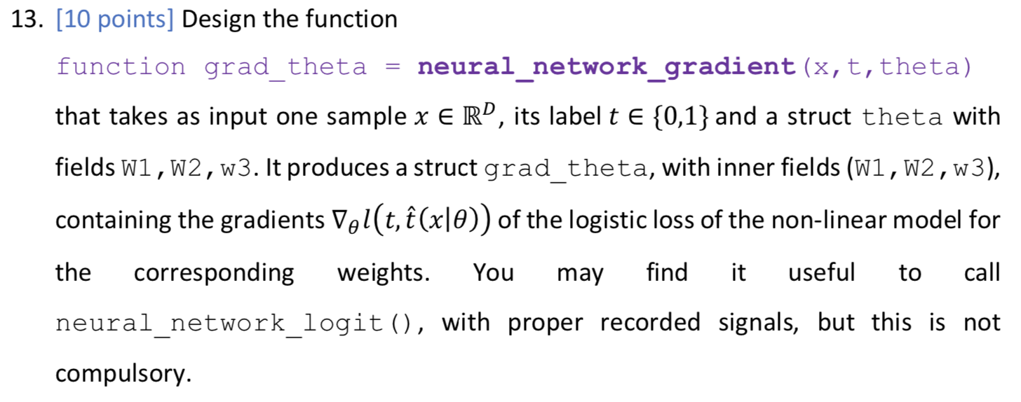
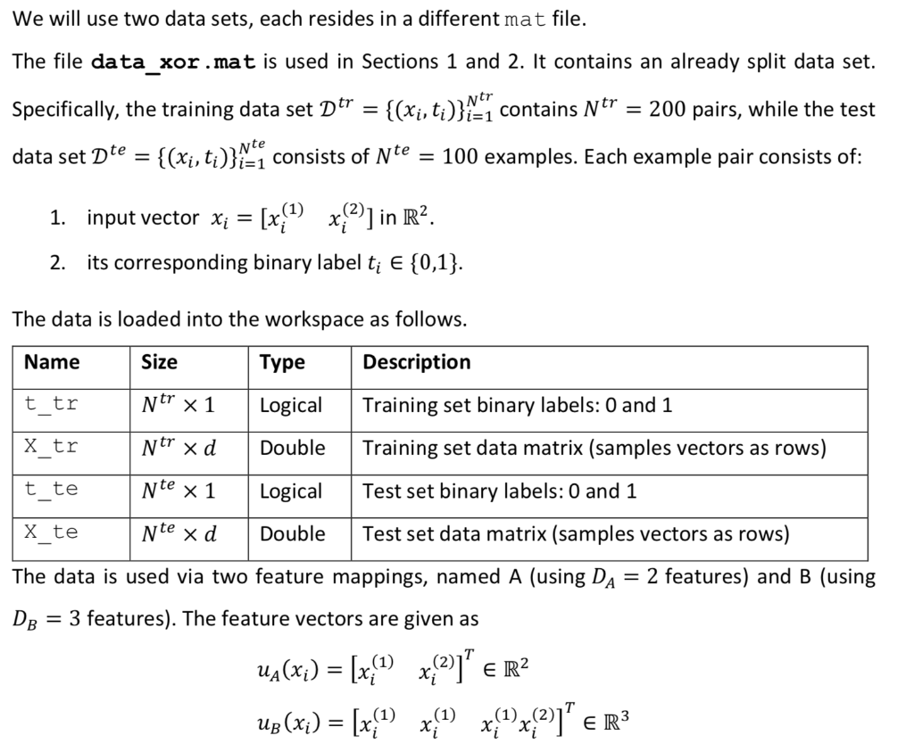
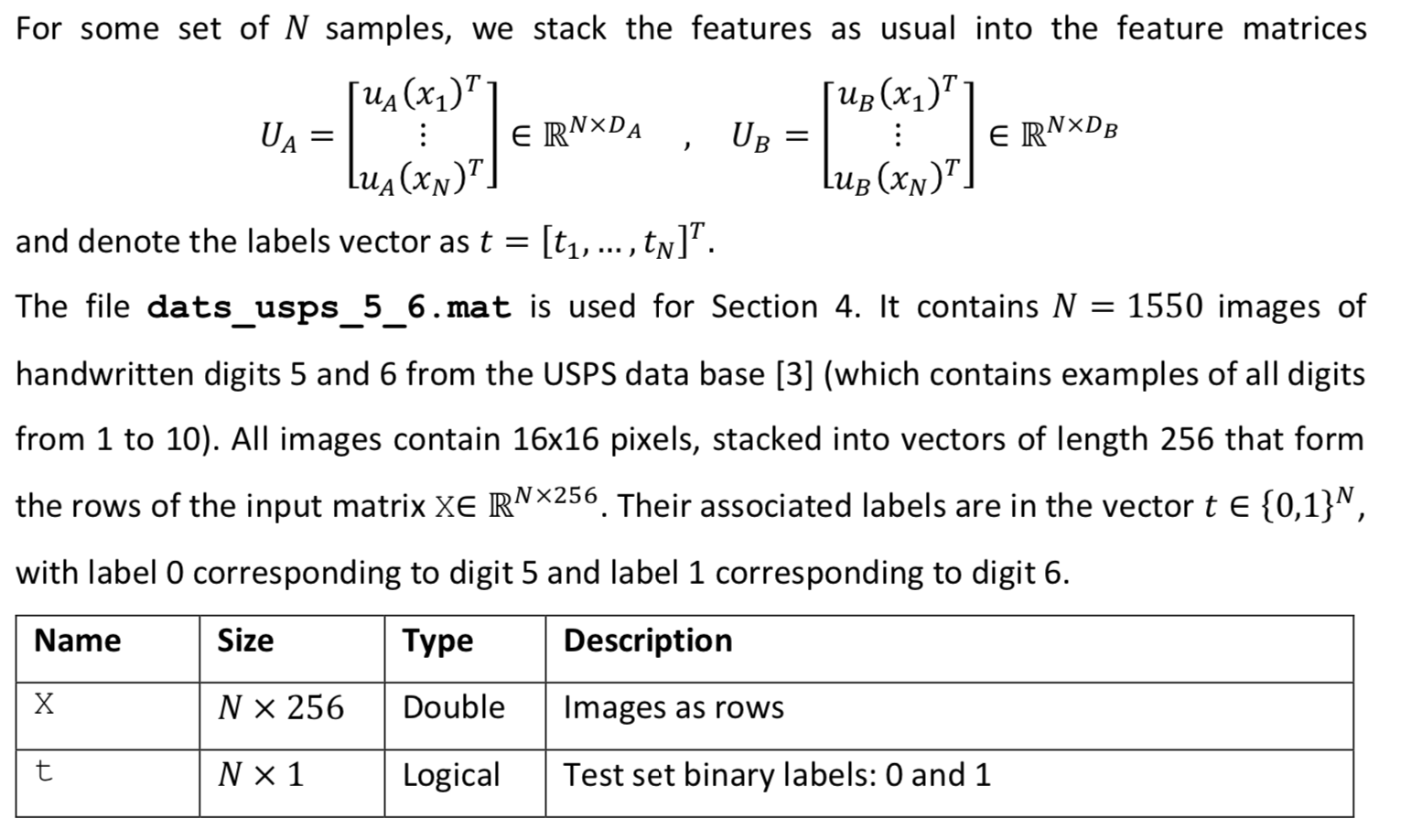
We now consider a 3-layer neural network model for binary classification, with input features of size D, number of neurons in the first hidden layer D, and in the second hidden layer D2, = and ReLU activation in the hidden layers. To represent the model parameters 0 {W1,w2, w3}, we use a MATLAB struct [2] to group the matrices. The model parameters can be accessed using the struct fields. For a struct named theta, use theta.W1, theta.W2 and theta.w3 to access them as regular variables. The functions to be designed must be written to account for general layer sizes, for 3-layer neural networks. You can assume the number of layers is 3, without generalizing it. We use the lectures notations and denote the input features as x rather than u as in the previous sections. This section does not use any data set. The main body calls for the listed function for two different input feature vectors, using the same model parameter vector 0 as provided within the main body. 11. [5 points] Design the function function [logit, record]= neural_network_logit (x, theta) that takes as inputs a single feature vector x E RD and a model parameter theta. = The function returns the logit logiteR of a neural network with feature vector u. You may use the second output record as a structure with fields of your choice, to record inner variables that can be useful when designing the upcoming function neural_network_gradient(). This structure is not marked, you can leave it empty before you reach designing the next function, or if it isn't useful for you even after. You may use the function ReLU(), as provided in the auxiliary functions. 12. [5 points] Design the function function out= grad_RELU (in) that computes entry-wise the gradient of the non linear activation function Relu over any size vector or matrix in, outputting a vector or matrix out of the same size. As it is not defined when an input entry is 0, we choose arbitrarily for this case the output to be 0. 13. [10 points] Design the function function grad_theta = neural_network_gradient (x, t, theta) that takes as input one sample x e R, its label t {0,1} and a struct theta with fields W1,W2, W3. It produces a struct grad_theta, with inner fields (W1,W2,w3), containing the gradients Vollt, (x|0)) of the logistic loss of the non-linear model for I the corresponding weights. You may find it useful to call neural_network_logit (), with proper recorded signals, but this is not compulsory. We will use two data sets, each resides in a different mat file. Ntr The file data_xor.mat is used in Sections 1 and 2. It contains an already split data set. Specifically, the training data set D tr {(Xisti)}; contains Ntr = 200 pairs, while the test data set Dte {(xi,ti)}=1 consists of Nte = 100 examples. Each example pair consists of: = 1) 1. input vector xi = [x{1 x??)] in R2. 2. its corresponding binary label ti E {0,1}. The data is loaded into the workspace as follows. Name Size Type Description t tr Ntr x1 Logical Training set binary labels: 0 and 1 X tr Ntr xd Double Training set data matrix (samples vectors as rows) t te Nte x 1 Logical Test set binary labels: 0 and 1 X te Nte xd Double Test set data matrix (samples vectors as rows) The data is used via two feature mappings, named A (using Da = 2 features) and B (using DB = 3 features). The feature vectors are given as () Ug(x;) = [x{1} {{2))"ER2 Up (x;) = [x{1} {{1x