please do not change the variables that are already written in the questions or the seed (if any is given).

All code must be executable from scratch. Code should be written properly (i.e. put code in functions as needed, declare variables as needed, and don't repeat yourself.) Only use functions from the packages loaded in the first block of code below for this problem set.

Make sure all plots contain appropriately labelled axes and are easy to read and interpret.

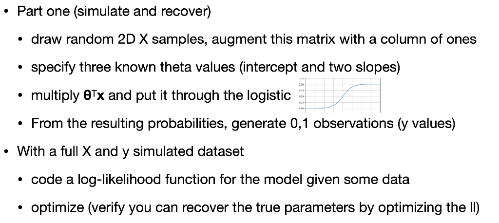
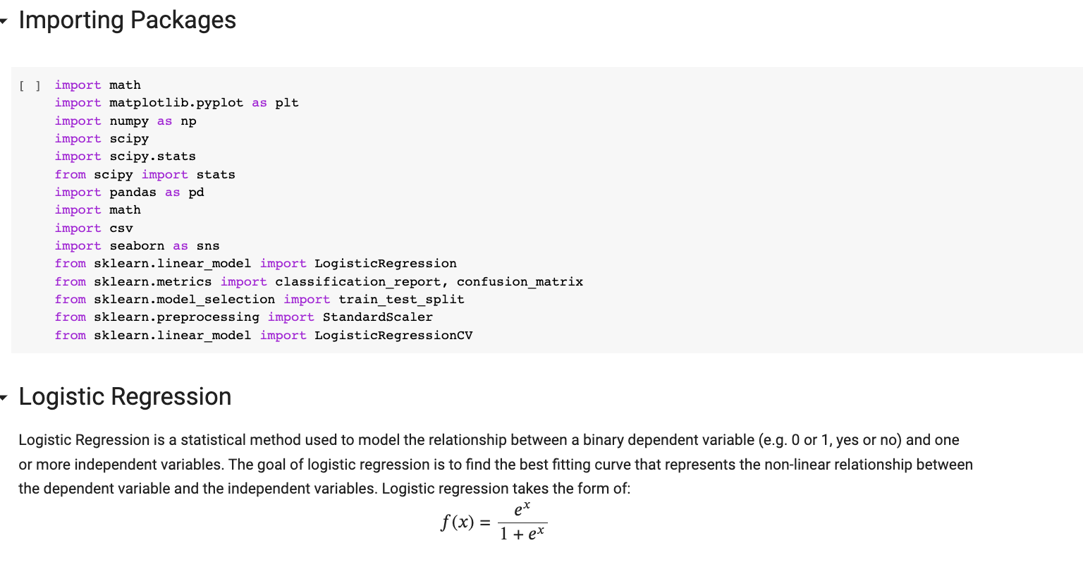
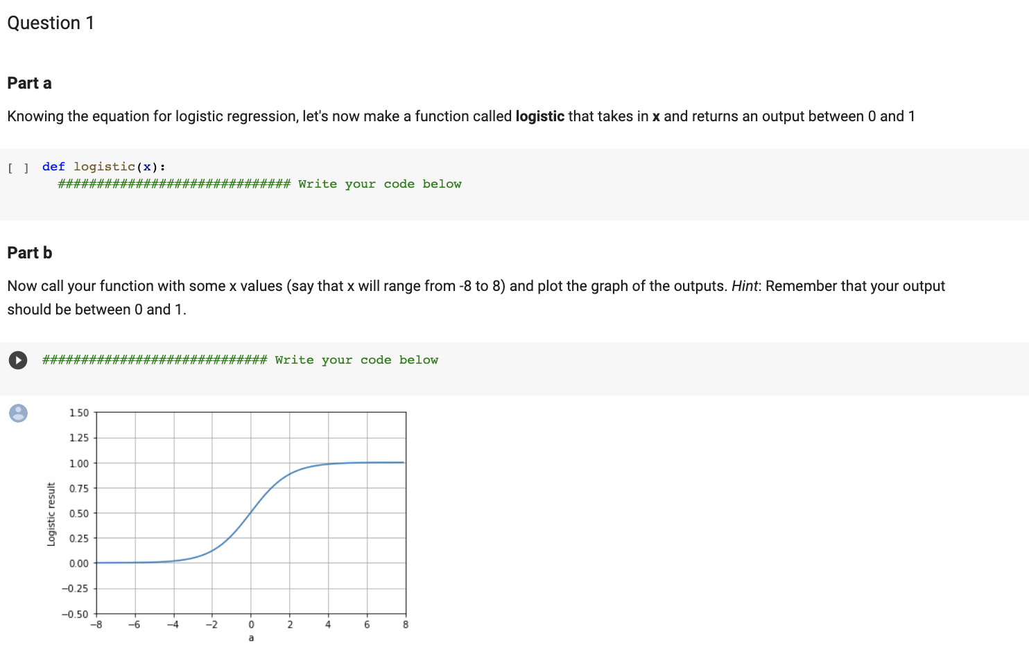
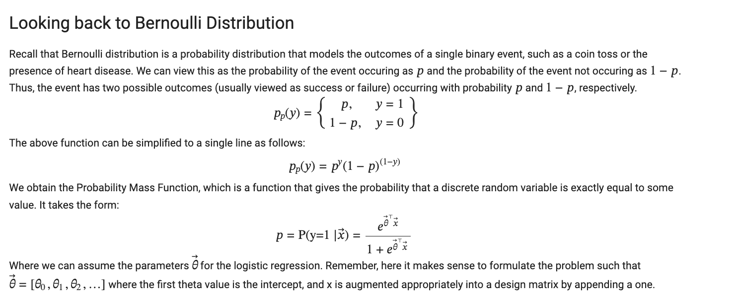
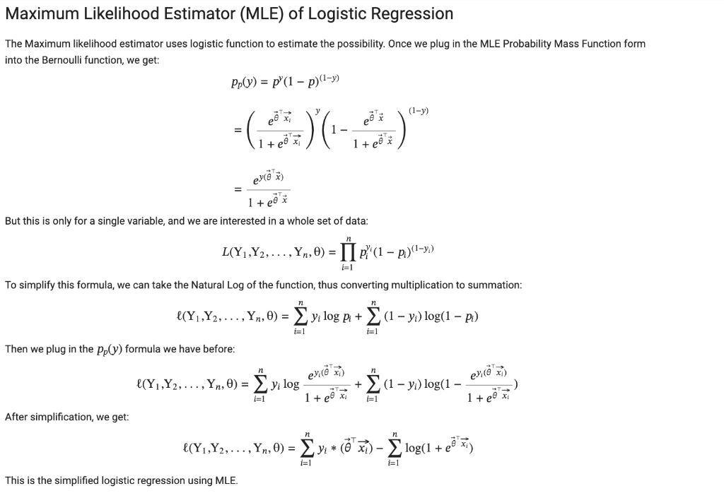
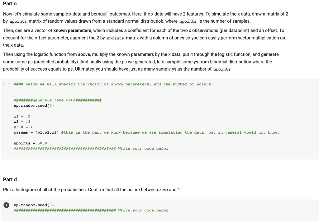
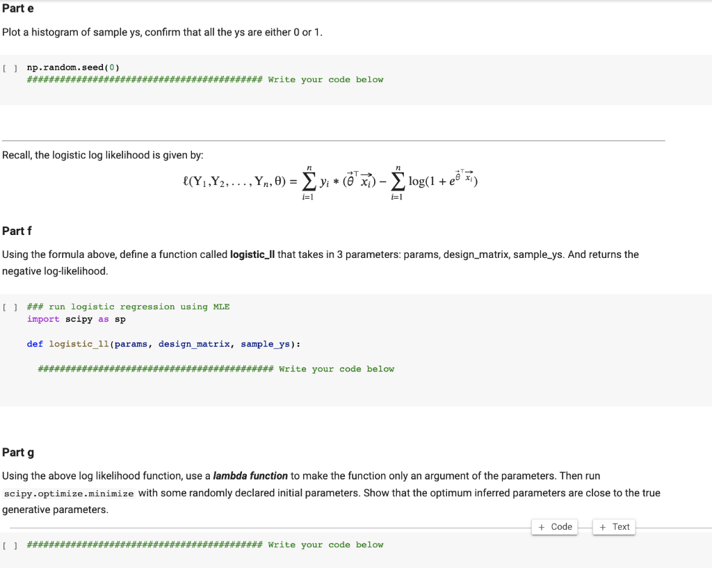
- Part one (simulate and recover) - draw random 2D X samples, augment this matrix with a column of ones - specify three known theta values (intercept and two slopes) - multiply x and put it through the logistic - From the resulting probabilities, generate 0,1 observations ( y values) - With a full X and y simulated dataset - code a log-likelihood function for the model given some data - optimize (verify you can recover the true parameters by optimizing the Il) Importing Packages [ ] import math import matplotlib.pyplot as plt import numpy as np import scipy import scipy.stats from scipy import stats import pandas as pd import math import csv import seaborn as sns from sklearn.linear_model import Logistickegression from sklearn.metrics import classification_report, confusion_matrix from sklearn.model_selection import train_test_split from sklearn.preprocessing import StandardScaler from sklearn.linear_model import LogistickegressioncV Logistic Regression Logistic Regression is a statistical method used to model the relationship between a binary dependent variable (e.g. 0 or 1 , yes or no) and one or more independent variables. The goal of logistic regression is to find the best fitting curve that represents the non-linear relationship between the dependent variable and the independent variables. Logistic regression takes the form of: f(x)=1+exex Part a Knowing the equation for logistic regression, let's now make a function called logistic that takes in x and returns an output between 0 and 1 [ ] def logistic (x): \#\#\#\#\#\#\#\#\#\#\#\#\#\#\#\#\#\#\#\#\#\#\#\#\#\#\#\#\#\# Write your code below Part b Now call your function with some x values (say that x will range from 8 to 8 ) and plot the graph of the outputs. Hint: Remember that your output should be between 0 and 1 . \#\#\#\#\#\#\#\#\#\#\#\#\#\#\#\#\#\#\#\#\#\#\#\#\#\#\#\#\# write your code below Looking back to BernoullI Distribution Recall that Bernoulli distribution is a probability distribution that models the outcomes of a single binary event, such as a coin toss or the presence of heart disease. We can view this as the probability of the event occuring as p and the probability of the event not occuring as 1p. Thus, the event has two possible outcomes (usually viewed as success or failure) occurring with probability p and 1p, respectively. pp(y)={p,1p,y=1y=0} The above function can be simplified to a single line as follows: pp(y)=py(1p)(1y) We obtain the Probability Mass Function, which is a function that gives the probability that a discrete random variable is exactly equal to some value. It takes the form: p=P(y=1x)=1+exex Where we can assume the parameters for the logistic regression. Remember, here it makes sense to formulate the problem such that =[0,1,2,] where the first theta value is the intercept, and x is augmented appropriately into a design matrix by appending a one. The Maximum likelihood estimator uses logistic function to estimate the possibility. Once we plug in the MLE Probability Mass Function form into the Bernoulli function, we get: pp(y)=py(1p)(1y)=(1+exiexi)y(11+exex)(1y)=1+exey(x) But this is only for a single variable, and we are interested in a whole set of data: L(Y1,Y2,,Yn,)=i=1npiyi(1pi)(1yi) To simplify this formula, we can take the Natural Log of the function, thus converting multiplication to summation: (Y1,Y2,,Yn,)=i=1nyilogpi+i=1n(1yi)log(1pi) Then we plug in the pp(y) formula we have before: (Y1,Y2,,Yn,)=i=1nyilog1+exieyi(xi)+i=1n(1yi)log(11+exieyi(xi)) After simplification, we get: (Y1,Y2,,Yn,)=i=1nyi(xi)i=1nlog(1+exi) This is the simplified logistic regression using MLE. Now let's simulate some sample x data and bernoulli outcomes. Here, the x data will have 2 features. To simulate the x data, draw a matrix of 2 by npoints matrix of random values drawn from a standard normal distributiob, where npoints is the number of samples. Then, declare a vector of known parameters, which includes a coefficient for each of the two x observations (per datapoint) and an offset. To account for the offset parameter, augment the 2 by npoints matrix with a column of ones so you can easily perform vector multiplication on the x data. Then using the logistic function from above, multiply the known parameters by the x data, put it through the logistic function, and generate some some ps (predicted probability). And finally using the ps we generated, lets sample some ys from binomial distribution where the probability of success equals to ps. Ultimatey, you should have just as many sample ys as the number of npoints . [ ] \#\#\#\# below we will specify the vector of known parameters, and the number of points. \#\#\#\#\#\#\#\#generate fake datan\#\#\#\#\#\#\#\#\#\#\# np.random. seed (0) w1=.2 w2=.8 w3=.4 params =[w1,w2,w3] \#this is the part we know because we are simulating the data, but in general would not know npoints =5000 \#\#\#\#\#\#\#\#\#\#\#\#\#\#\#\#\#\#\#\#\#\#\#\#\#\#\#\#\#\#\#\#\#\#\#\#\#\#\#\#\#\#\#\#\#\#\# write your code below Part d Plot a histogram of all of the probabilities. Confirm that all the ps are between zero and 1. np.random. seed (0) \#\#\#\#\#\#\#\#\#\#\#\#\#\#\#\#\#\#\#\#\#\#\#\#\#\#\#\#\#\#\#\#\#\#\#\#\#\#\#\#\#\#\#\#\# write your code below [ ] np.random. seed(0) \#\#\#\#\#\#\#\#\#\#\#\#\#\#\#\#\#\#\#\#\#\#\#\#\#\#\#\#\#\#\#\#\#\#\#\#\#\#\#\#\#\#\# write your code below Recall, the logistic log likelihood is given by: (Y1,Y2,,Yn,)=i=1nyi(xi)i=1nlog(1+exi) Part f Using the formula above, define a function called logistic_Il that takes in 3 parameters: params, design_matrix, sample_ys. And returns the negative log-likelihood. [] \#\#\# run logistic regression using MLE import scipy as sp def logistic_ll(params, design_matrix, sample_ys): \#\#\#\#\#\#\#\#\#\#\#\#\#\#\#\#\#\#\#\#\#\#\#\#\#\#\#\#\#\#\#\#\#\#\#\#\#\#\#\#\#\#\# write your code below Part g Using the above log likelihood function, use a lambda function to make the function only an argument of the parameters. Then run scipy . optimize.minimize with some randomly declared initial parameters. Show that the optimum inferred parameters are close to the true generative parameters