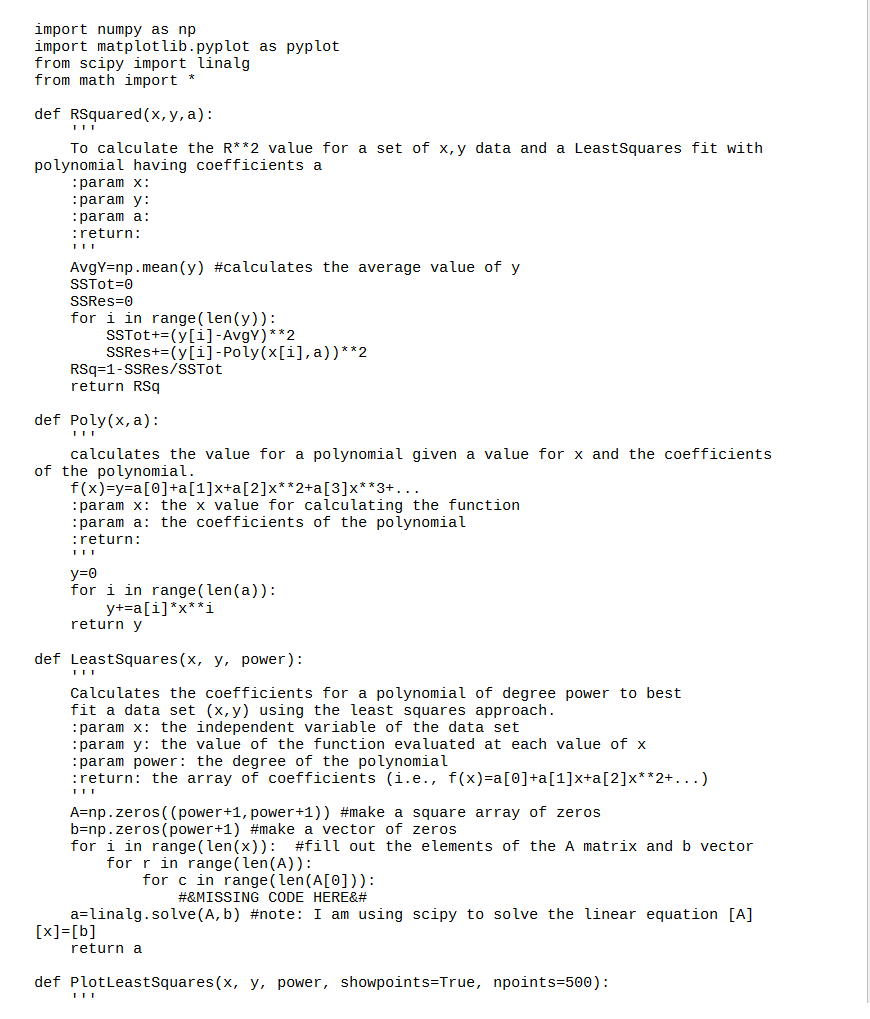
please fill in missing code

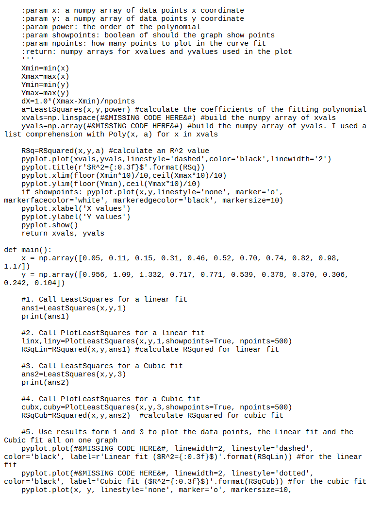
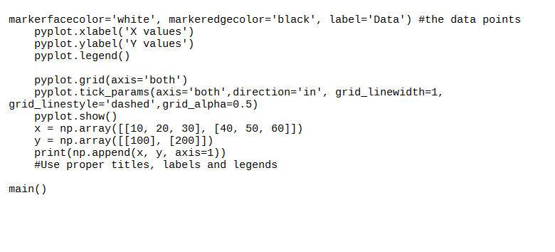
import numpy as np import matplot lib.pyplot as pyplot from scipy import linalg from math import * def RSquared(x,y,a): To calculate the R**2 value for a set of x,y data and a Least Squares fit with polynomial having coefficients a :param x: :param y: :param a: :return: AvgY=np.mean(y) #calculates the average value of y SSTot=0 SSRes=0 for i in range (len(y)): SSTot+=(y[i] -AvgY)**2 SSRes+=(y[i]-Poly(x[i], a))**2 RSq=1 - SSRes/SSTOL return RS def Poly(x,a): calculates the value for a polynomial given a value for x and the coefficients of the polynomial. f(x)=y=a[0]+a[1]x+a[2]***2+a[3]x**3+... :param x: the x value for calculating the function :param a: the coefficients of the polynomial :return: y=0 for i in range(len(a)): y+=a[i]*x**i return y def Least Squares (x, y, power): Calculates the coefficients for a polynomial of degree power to best fit a data set (x,y) using the least squares approach. :param x: the independent variable of the data set param y: the value of the function evaluated at each value of x :param power: the degree of the polynomial return: the array of coefficients (i.e., f(x)=a[O]+a[1]x+a[2]***2+...) A=np.zeros((power+1, power+1)) #make a square array of zeros b=np.zeros(power+1) #make a vector of zeros for i in range(len(x)): #fill out the elements of the A matrix and b vector for r in range (len(A)): for c in range (len(A[0])): #&MISSING CODE HERE a=linalg. solve(A,b) #note: I am using scipy to solve the linear equation [A] [x]=[b] return a def PlotLeast squares (x, y, power, showpoints=True, npoints=500): param x: a numpy array of data points x coordinate :param y: a numpy array of data points y coordinate :param power: the order of the polynomial param showpoints: boolean of should the graph show points :param npoints: how many points to plot in the curve fit :return: numpy arrays for xvalues and yvalues used in the plot Xmin=min(x) Xmax=max(x) Ymin=min(y) Ymax=max(y) dX=1.0*(Xmax-Xmin)points a=Least Squares (x, y, power) #calculate the coefficients of the fitting polynomial xvals=np. linspace(#&MISSING CODE HERE) #build the numpy array of xvals yvals=np.array(#&MISSING CODE HERE) #build the numpy array of yvals. I used a list comprehension with Poly(x, a) for x in xvals RSq=RSquared(x, y, a) #calculate an R^2 value pyplot.plot(xvals, yvals, linestyle='dashed', color='black', linewidth='2') pyplot.title(r'$R^2={:0.3f}$'.format(RSq)) pyplot.xlim(floor(Xmin*10)/10, ceil(Xmax*10)/10) pyplot.ylim(floor(min), ceil(Ymax*10)/10) if showpoints: pyplot.plot(x, y, linestyle='none', marker='0', markerfacecolor='white', markeredgecolor='black', markersize=10) pyp lot.xlabel('x values') pyplot.y label('Y values') pyp lot. show return xvals, yvals def main(): x = np.array( [0.05, 0.11, 0.15, 0.31, 0.46, 0.52, 0.70, 0.74, 0.82, 0.98, 1.17]) y = np.array([0.956, 1.09, 1.332, 0.717, 0.771, 0.539, 0.378, 0.370, 0.306, 0.242, 0.104]) #1. Call Least Squares for a linear fit ans1=Least Squares(x, y, 1) print(ans1) #2. Call PlotLeast Squares for a linear fit linx, liny=PlotLeast Squares(x,y,1, showpoints=True, npoints=500) RSqLin=RSquared(x, y, ans1) #calculate RSqured for linear fit #3. Call Least Squares for a Cubic fit ans2=Least Squares (x, y,3) print(ans2) #4. Call PlotLeast squares for a Cubic fit cubx, cuby=PlotLeast Squares(x,y,3, showpoints=True, npoints=500) RSqCub=Rsquared(x, y, ans2) #calculate RSquared for cubic fit #5. Use results form 1 and 3 to plot the data points, the Linear fit and the Cubic fit all on one graph pyplot.plot(#&MISSING CODE HERE, linewidth=2, linestyle='dashed', color='black', label=r 'Linear fit ($R^2={:0.3f}$)'.format(RSqLin)) #for the linear fit pyplot.plot(#&MISSING CODE HERE, linewidth=2, linestyle='dotted', color='black', label='Cubic fit ($R^2={:0.3f}$)'.format(RSqCub)) #for the cubic fit pyplot.plot(x, y, linestyle='none', marker='o', markersize=10, markerfacecolor='white', markeredgecolor='black', label='Data') #the data points pyplot.xlabel('x values') pyplot.ylabel('Y values') pyplot. legend() pyplot.grid(axis='both') pyplot.tick_params (axis='both', direction='in', grid_linewidth=1, grid_linestyle='dashed',grid_alpha=0.5) pyplot.show() x = np.array([[10, 20, 30], [40, 50, 60]]) y = np.array([[100], [200]]) print(np.append(x, y, axis=1)) Use proper ti labels and legends main() import numpy as np import matplot lib.pyplot as pyplot from scipy import linalg from math import * def RSquared(x,y,a): To calculate the R**2 value for a set of x,y data and a Least Squares fit with polynomial having coefficients a :param x: :param y: :param a: :return: AvgY=np.mean(y) #calculates the average value of y SSTot=0 SSRes=0 for i in range (len(y)): SSTot+=(y[i] -AvgY)**2 SSRes+=(y[i]-Poly(x[i], a))**2 RSq=1 - SSRes/SSTOL return RS def Poly(x,a): calculates the value for a polynomial given a value for x and the coefficients of the polynomial. f(x)=y=a[0]+a[1]x+a[2]***2+a[3]x**3+... :param x: the x value for calculating the function :param a: the coefficients of the polynomial :return: y=0 for i in range(len(a)): y+=a[i]*x**i return y def Least Squares (x, y, power): Calculates the coefficients for a polynomial of degree power to best fit a data set (x,y) using the least squares approach. :param x: the independent variable of the data set param y: the value of the function evaluated at each value of x :param power: the degree of the polynomial return: the array of coefficients (i.e., f(x)=a[O]+a[1]x+a[2]***2+...) A=np.zeros((power+1, power+1)) #make a square array of zeros b=np.zeros(power+1) #make a vector of zeros for i in range(len(x)): #fill out the elements of the A matrix and b vector for r in range (len(A)): for c in range (len(A[0])): #&MISSING CODE HERE a=linalg. solve(A,b) #note: I am using scipy to solve the linear equation [A] [x]=[b] return a def PlotLeast squares (x, y, power, showpoints=True, npoints=500): param x: a numpy array of data points x coordinate :param y: a numpy array of data points y coordinate :param power: the order of the polynomial param showpoints: boolean of should the graph show points :param npoints: how many points to plot in the curve fit :return: numpy arrays for xvalues and yvalues used in the plot Xmin=min(x) Xmax=max(x) Ymin=min(y) Ymax=max(y) dX=1.0*(Xmax-Xmin)points a=Least Squares (x, y, power) #calculate the coefficients of the fitting polynomial xvals=np. linspace(#&MISSING CODE HERE) #build the numpy array of xvals yvals=np.array(#&MISSING CODE HERE) #build the numpy array of yvals. I used a list comprehension with Poly(x, a) for x in xvals RSq=RSquared(x, y, a) #calculate an R^2 value pyplot.plot(xvals, yvals, linestyle='dashed', color='black', linewidth='2') pyplot.title(r'$R^2={:0.3f}$'.format(RSq)) pyplot.xlim(floor(Xmin*10)/10, ceil(Xmax*10)/10) pyplot.ylim(floor(min), ceil(Ymax*10)/10) if showpoints: pyplot.plot(x, y, linestyle='none', marker='0', markerfacecolor='white', markeredgecolor='black', markersize=10) pyp lot.xlabel('x values') pyplot.y label('Y values') pyp lot. show return xvals, yvals def main(): x = np.array( [0.05, 0.11, 0.15, 0.31, 0.46, 0.52, 0.70, 0.74, 0.82, 0.98, 1.17]) y = np.array([0.956, 1.09, 1.332, 0.717, 0.771, 0.539, 0.378, 0.370, 0.306, 0.242, 0.104]) #1. Call Least Squares for a linear fit ans1=Least Squares(x, y, 1) print(ans1) #2. Call PlotLeast Squares for a linear fit linx, liny=PlotLeast Squares(x,y,1, showpoints=True, npoints=500) RSqLin=RSquared(x, y, ans1) #calculate RSqured for linear fit #3. Call Least Squares for a Cubic fit ans2=Least Squares (x, y,3) print(ans2) #4. Call PlotLeast squares for a Cubic fit cubx, cuby=PlotLeast Squares(x,y,3, showpoints=True, npoints=500) RSqCub=Rsquared(x, y, ans2) #calculate RSquared for cubic fit #5. Use results form 1 and 3 to plot the data points, the Linear fit and the Cubic fit all on one graph pyplot.plot(#&MISSING CODE HERE, linewidth=2, linestyle='dashed', color='black', label=r 'Linear fit ($R^2={:0.3f}$)'.format(RSqLin)) #for the linear fit pyplot.plot(#&MISSING CODE HERE, linewidth=2, linestyle='dotted', color='black', label='Cubic fit ($R^2={:0.3f}$)'.format(RSqCub)) #for the cubic fit pyplot.plot(x, y, linestyle='none', marker='o', markersize=10, markerfacecolor='white', markeredgecolor='black', label='Data') #the data points pyplot.xlabel('x values') pyplot.ylabel('Y values') pyplot. legend() pyplot.grid(axis='both') pyplot.tick_params (axis='both', direction='in', grid_linewidth=1, grid_linestyle='dashed',grid_alpha=0.5) pyplot.show() x = np.array([[10, 20, 30], [40, 50, 60]]) y = np.array([[100], [200]]) print(np.append(x, y, axis=1)) Use proper ti labels and legends main()