please follow the steps to solve Excel

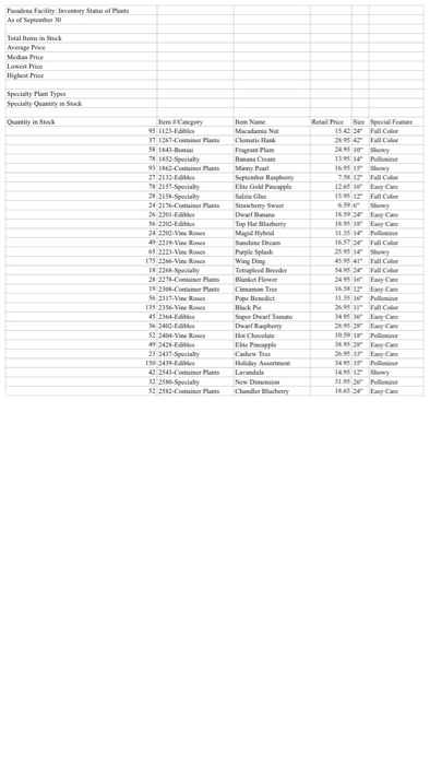
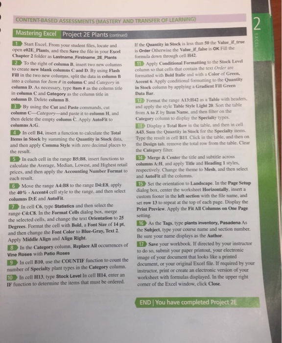
Pasadena Facility every Saofants Total om in Stock Average Price Medias Price Ilighet Fries Specialty Plant Type Specialty Quantity in Stock C Macadamia Nut atis Hank Fragrantum 15.4 5 Full Color Fall Color 1395 Pollici 1695 15" Show September Rasphemy Elite P apple 12.05 16 Easy Care Sawberry Sweet 18.39 1805 11351 Easy Care Easy Care Pati 65 2223-Wine Roses 45 95 41" Fall Color Full Color 56 231 7. Viss 115 211 Views 10:35 16" Pollir 11 Full Color 34,95 36 ayad Dwarf Rashery 10:59 49 249 EAN 3 Ewy Plants 42 2543-C 52 253 Specialty 31.52" Police 18. Bay CONTENT-BASED ASSESSMENTS (MASTERY AND TRANSFER OF LEARNING) N EXCEL Mastering Excel Project 2E Plants (continued 1 Start Excel. From your student files, locate and open co2E Plants, and then Save the file in your wall Chapter 2 folder as Lastname Firstname 2E Plants 2 To the right of column B, insert two new columns to create new blank columns C and D. By using Flash Fill in the two new columns, split the data in column B into a column for lem in column C and Category in column D. As necessary, type Item # as the column title in column C and Category as the column title in column D. Delete column B. 3 By using the Cut and Paste commands, cut column C Category and paste it to column H. and then delete the empty column C. Apply AutoFit to columns A:G 4 In cell B4, insert a function to calculate the Total Items in Stock by summing the Quantity in Stock data, and then apply Comma Style with zero decimal places to the result. 5 In each cell in the range B5:38, insert functions to calculate the Average, Median, Lowest, and Highest retail prices, and then apply the Accounting Number Format to each result. 6 Move the range A4:38 to the range D4:E8, apply the 40% - Accent4 cell style to the range, and then select columns D:E and AutoFit. 7 In cell C6, type Statistics and then select the range C4:08. In the Format Cells dialog box, merge the selected cells, and change the text Orientation to 25 Degrees. Format the cell with Bold, a Font Size of 14 pt. and then change the Font Color to Blue-Gray, Text 2 Apply Middle Align and Align Right. 8 In the Category column, Replace All occurrences of Vine Roses with Patio Roses 9 In cell B10, use the COUNTIF function to count the number of Specialty plant types in the Category column. 10 In cell H13, type Stock Level In cell H14, enter an IF function to determine the items that must be ordered If the Quantity in Stock is less than 50 the Value_iftrue is Order Otherwise the value if false is OK Fill the formula down through cell H42 11 Apply Conditional Formatting to the Stock Level column so that cells that contain the text Onder are formatted with Bold Italic and with a Color of Green, Accent 6. Apply conditional formatting to the Quantity in Stock column by applying a Gradient Full Green Data Bar. 12 Format the range A13:42 as a Table with headers. and apply the style Table Style Light 20. Sort the table from A to Z by Item Name, and then filter on the Category column to display the Specialty types Display a Total Row in the table, and then in cell A43, Sum the Quantity in Stock for the Specialty items. Type the result in cell B1. Click in the table, and then on the Design tab, remove the total row from the table. Clear the Category filter. 14 Merge & Center the title and subtitle across columns A:H, and apply Title and Heading 1 styles. respectively. Change the theme to Mesh, and then select and AutoFit all the columns. 15 Set the orientation to Landscape. In the Page Setup dialog box, center the worksheet Horizontally, insert a custom footer in the left section with the file name, and set row 13 to repeat at the top of each page. Display the Print Preview. Apply the Fit All Columns on One Page setting 16 As the Tags, type plants inventory, Pasadena As the Subject, type your course name and section number. Be sure your name displays as the Author. 17 Save your workbook. If directed by your instructor to do so, submit your paper printout, your electronic image of your document that looks like a printed document, or your original Excel file. If required by your instructor, print or create an electronic version of your worksheet with formulas displayed. In the upper right corner of the Excel window, click Close. END | You have completed Project 2E Pasadena Facility every Saofants Total om in Stock Average Price Medias Price Ilighet Fries Specialty Plant Type Specialty Quantity in Stock C Macadamia Nut atis Hank Fragrantum 15.4 5 Full Color Fall Color 1395 Pollici 1695 15" Show September Rasphemy Elite P apple 12.05 16 Easy Care Sawberry Sweet 18.39 1805 11351 Easy Care Easy Care Pati 65 2223-Wine Roses 45 95 41" Fall Color Full Color 56 231 7. Viss 115 211 Views 10:35 16" Pollir 11 Full Color 34,95 36 ayad Dwarf Rashery 10:59 49 249 EAN 3 Ewy Plants 42 2543-C 52 253 Specialty 31.52" Police 18. Bay CONTENT-BASED ASSESSMENTS (MASTERY AND TRANSFER OF LEARNING) N EXCEL Mastering Excel Project 2E Plants (continued 1 Start Excel. From your student files, locate and open co2E Plants, and then Save the file in your wall Chapter 2 folder as Lastname Firstname 2E Plants 2 To the right of column B, insert two new columns to create new blank columns C and D. By using Flash Fill in the two new columns, split the data in column B into a column for lem in column C and Category in column D. As necessary, type Item # as the column title in column C and Category as the column title in column D. Delete column B. 3 By using the Cut and Paste commands, cut column C Category and paste it to column H. and then delete the empty column C. Apply AutoFit to columns A:G 4 In cell B4, insert a function to calculate the Total Items in Stock by summing the Quantity in Stock data, and then apply Comma Style with zero decimal places to the result. 5 In each cell in the range B5:38, insert functions to calculate the Average, Median, Lowest, and Highest retail prices, and then apply the Accounting Number Format to each result. 6 Move the range A4:38 to the range D4:E8, apply the 40% - Accent4 cell style to the range, and then select columns D:E and AutoFit. 7 In cell C6, type Statistics and then select the range C4:08. In the Format Cells dialog box, merge the selected cells, and change the text Orientation to 25 Degrees. Format the cell with Bold, a Font Size of 14 pt. and then change the Font Color to Blue-Gray, Text 2 Apply Middle Align and Align Right. 8 In the Category column, Replace All occurrences of Vine Roses with Patio Roses 9 In cell B10, use the COUNTIF function to count the number of Specialty plant types in the Category column. 10 In cell H13, type Stock Level In cell H14, enter an IF function to determine the items that must be ordered If the Quantity in Stock is less than 50 the Value_iftrue is Order Otherwise the value if false is OK Fill the formula down through cell H42 11 Apply Conditional Formatting to the Stock Level column so that cells that contain the text Onder are formatted with Bold Italic and with a Color of Green, Accent 6. Apply conditional formatting to the Quantity in Stock column by applying a Gradient Full Green Data Bar. 12 Format the range A13:42 as a Table with headers. and apply the style Table Style Light 20. Sort the table from A to Z by Item Name, and then filter on the Category column to display the Specialty types Display a Total Row in the table, and then in cell A43, Sum the Quantity in Stock for the Specialty items. Type the result in cell B1. Click in the table, and then on the Design tab, remove the total row from the table. Clear the Category filter. 14 Merge & Center the title and subtitle across columns A:H, and apply Title and Heading 1 styles. respectively. Change the theme to Mesh, and then select and AutoFit all the columns. 15 Set the orientation to Landscape. In the Page Setup dialog box, center the worksheet Horizontally, insert a custom footer in the left section with the file name, and set row 13 to repeat at the top of each page. Display the Print Preview. Apply the Fit All Columns on One Page setting 16 As the Tags, type plants inventory, Pasadena As the Subject, type your course name and section number. Be sure your name displays as the Author. 17 Save your workbook. If directed by your instructor to do so, submit your paper printout, your electronic image of your document that looks like a printed document, or your original Excel file. If required by your instructor, print or create an electronic version of your worksheet with formulas displayed. In the upper right corner of the Excel window, click Close. END | You have completed Project 2E