

Question: Please help! 1 . In the Gradebook Math worksheet, use Advanced Filter to find students who had less than 8 0 on the midterm or
Please help!
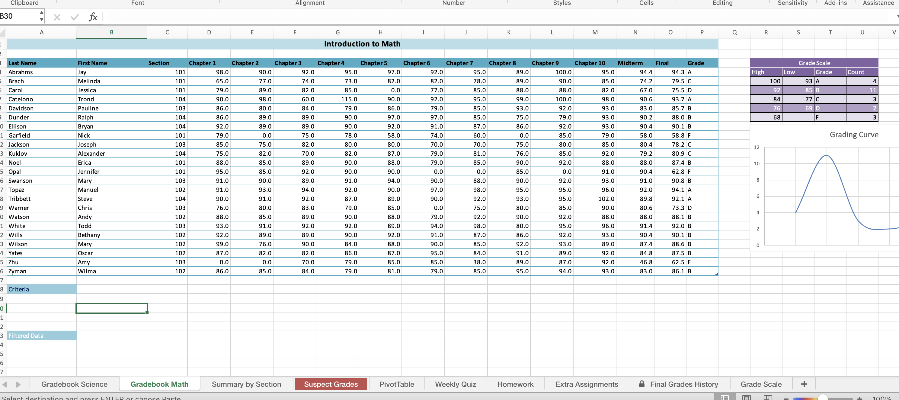
In the Gradebook Math worksheet, use Advanced Filter to find students who had less than on the
midterm or had less than on the final. Copy cells A:P and paste them starting in cell A for use as
the header row in the criteria range. Enter the criteria range to find rows where the value in the Midterm
column is or the value in the Final column is Use Advanced Filter and copy the filtered data to
the range beginning with cell A
In the Summary by Section worksheet, use Consolidate to create a summary of the grades by section.
Place the summary in cell A of the Summary by Section worksheet. Use the Average function.
Consolidate data from the cell range C:O in the Gradebook Math worksheet. Use labels from both the
top row and the left column. Do not create links to the source data. Autofit the columns, if necessary. On
the Summary by Section worksheet, center and merge the title across cells A:M
In the Suspect Grades worksheet, apply conditional formatting to find suspicious grades duplicate values
for each assignment Red, Accent and Bold formatting. You will need to create separate conditional
formatting rules one for each chapter assignment. Filter each of the columns to show only the cells with
the red font color.
Make the following updates in the PivotTable worksheet: Add a calculated field named Difference to
the PivotTable to calculate the difference between the final average and the midterm average for each
section; Apply the Pivot Style Medium Quick Style to the PivotTable; Change the PivotChart to a
combo chart with the Sum of Difference series as a line chart on the secondary axis and the other two
series as clustered column charts on the primary axis.; Apply the Style PivotChart Quick Style to the
PivotChart; Add a slicer to the PivotChart to filter the data by the Final field. If necessary, move the
slicer so it doesnt cover the PivotChart. Display data where the final exam scores are above only.
Step by Step Solution
There are 3 Steps involved in it
1 Expert Approved Answer
Step: 1 Unlock

Question Has Been Solved by an Expert!
Get step-by-step solutions from verified subject matter experts
Step: 2 Unlock
Step: 3 Unlock