Please help! im stuck

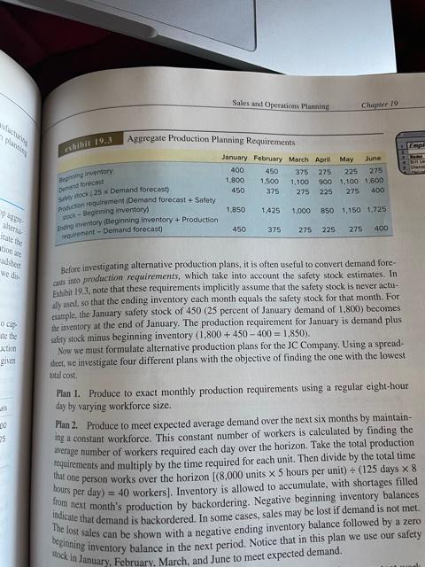
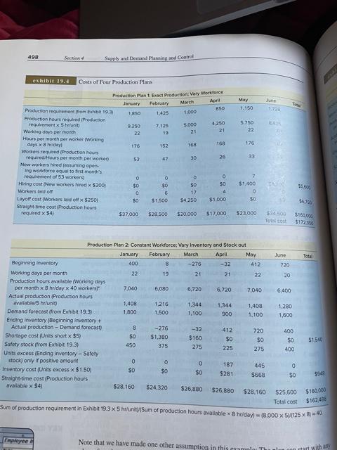
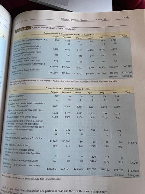
Using the data in Exhibit 19.3 prepare Excel Spreadsheets for each of the Production Plans( 1 to 4) shown in exhibit 19.4. In order to receive full credit you must use Excel Formulas for all calculation and you can only enter base case information once. .All additional uses of that information must be through use of a formula. Buonginey Beginning inventory + Production Stock25 Demand forecast) Porcon requirement (Demand forecast + Safety indicate that demand is backordered. In some cases, sales may be lost if demand is not met The lost sales can be shown with a negative ending inventory balance followed by a zero beginning inventory balance in the next period. Notice that in this plan we use our safety stock in January, February, March, and June to meet expected demand. Sales and Operation Planning Aggregate Production Planning Requirements January February March April May June 400 450 375 275 225 1,800 1,500 1.100 900 1.100 1.600 450 375 275 275 400 Chapter 19 Emp th 275 Bring Inventory Demand for 225 1.850 1.425 1.000 - Beginning inventory 850 1,150 1,725 2 essa 450 375 275 225 275 400 woent-Demand forecast, we - Ocas de the action given Before investigating alternative production plans, it is often useful to convert demand fore- es into production requirements, which take into account the safety stock estimates. In Exhibit 19.3.note that these requirements implicitly assume that the safety stock is never actu- ally used, so that the ending inventory each month equals the safety stock for that month. For cuample, the January safety stock of 450 (25 percent of January demand of 1,800) becomes the inventory at the end of January. The production requirement for January is demand plus safety stock minus beginning inventory (1,800 + 450 - 400 = 1,850). Now we must formulate alternative production plans for the JC Company. Using a spread- shect, we investigate four different plans with the objective of finding the one with the lowest Dital cost Plan 1. Produce to exact monthly production requirements using a regular eight-hour day by varying workforce size. Plan 2. Produce to meet expected average demand over the next six months by maintain- ing a constant workforce. This constant number of workers is calculated by finding the werage number of workers required each day over the horizon. Take the total production requirements and multiply by the time required for each unit. Then divide by the total time that one person works over the horizon (8,000 units x 5 hours per unit) + (125 days x 8 per day) = 40 workers). Inventory is allowed to accumulate, with shortages filled then next month's production by backordering. Negative beginning inventory balances 20 35 bours 498 Supply and Demand Planning and Control May 1.150 1.225 5.750 22 176 exhibit 19.4 Costs of Four Production Plans Production Plant Exact Production Vary Workforce January February March April Production requiremento Exhib 19.2 850 1850 1,000 Production hours required Production requirements 9,250 7.125 5.000 4.250 Working days per month 22. 19 21 21 Hours per month per worker (Working days x 8 heday 176 152 168 168 Workers required Production hours requred Hours per month per worker) 53 47 3D 26 New workers hired assuming open- Ing workforce equal to first month's requirement of 53 workers) 0 0 0 Hiring cost (New workers hired x $200 $0 $0 $0 Workers laid on 4 0 17 6 Layoff cost Workers laid of $250) $0 $1.500 $4,250 $1.000 Straight-time cost Production hours required x 34 $37.000 $28.500 $20.000 $17.000 OS 7 $1.400 0 SO 1550 16354 $23.000 534 Tottost $160.000 5172354 June Total 720 19 20 6,400 1,344 1.100 Production Plan 2: Constant Worldorce; Vary Inventory and Stock out January February March April May Beginning inventory 400 8 -276 -32 412 Working days per month 22 19 21 21 22 Production hours available (Working days per month x hday x 40 workers 7.040 5.080 6,720 6,720 7.040 Actual production Production hours available) 1,408 1,216 1.344 1,408 Demand forecast from Exhibit 19.3) 1.800 1,500 1.100 900 Ending inventory (Beginning inventory+ Actual production-Demand forecast 8 -276 -32 412 720 Shortage cost (Units short x $5) $0 $1,380 $160 $0 $0 Safety stock from Exhibit 19.3) 450 375 275 225 275 Units excess (Ending inventory - Safety stock only if positive amount 0 0 187 445 Inventory cost (Units excess x $1.50) $0 $0 $0 $668 Straight-time cost(Production hours available x $4) $28.160 $24,320 $26,880 $28,160 1.280 1,600 400 50 $1540 400 $281 0 $0 5949 $26.880 $25,600 Total cost $160.000 $162.488 Sum of production requirement in Exhibit 19.3 5 h/tySum of production hours available 8 heday) = 18,000 x 541125 x 8 = 40 Note that we have made one other assumption in this man tart with a Working Permined by trial and error See text for explanation Each of these lour plans focused on one particular cost, and the first three were simple pure 499 Costs of Four Production Plans concluded) Production Plan Constant Low Wow, Subcontract January February March 1.050 1.425 22 19 Total April 1.000 May 1.150 22 June 1725 20 21 21 4.400 3.100 4.200 4,600 4000 760 840 100 880 dictionary che Production Actual production 840 970 565 160 10 270 525 20 $19.400 $12.300 $3.200 560.000 5200 55,400 $18,500 Production hours * $17,600 $15.200 516,800 $16.000 517,600 $16.000 Total cos $100.000 $160.000 pronation requirement. In this example, Aprais minimum of 5 units. Number of workers required for Aprilis Total Productie Plan 4: Constant Workforce Overtime January February March April 400 177 22 19 21 554 22 June 792 20 21 con hours available Working days IX 38 workers aperin production Production hours 6,688 5,776 6.384 6.384 6.688 6,000 1,338 1.155 1.277 1.338 1216 1.800 1277 1.100 1,500 900 1.100 Onun frecast from Exhibit 193) Dat before overtime Beginning tay+Regular shift production Demand forecast. This number has been unded 10 ne nearest Integer -62 554 408 -345 375 177 0 62 792 0 0 0 $0 $0 $1,860 450 Dette counts overtime x 5 unit SEN Statystock rom bt 19.3) Otras Unt valable before Petite-Safety stock only positive $10,350 375 SO 275 $0 $12,210 225 275 400 0 329 517 0 $0 toy costiti excessive x $1.50 Becom Production hours avail 0 SO $0 $494 8 $12 $776 $1,281 $26.752 $23,104 $25,536 $25.536 $26.752 $24,320 Total cost $152.000 $165.491 Ohio Using the data in Exhibit 19.3 prepare Excel Spreadsheets for each of the Production Plans( 1 to 4) shown in exhibit 19.4. In order to receive full credit you must use Excel Formulas for all calculation and you can only enter base case information once. .All additional uses of that information must be through use of a formula. Buonginey Beginning inventory + Production Stock25 Demand forecast) Porcon requirement (Demand forecast + Safety indicate that demand is backordered. In some cases, sales may be lost if demand is not met The lost sales can be shown with a negative ending inventory balance followed by a zero beginning inventory balance in the next period. Notice that in this plan we use our safety stock in January, February, March, and June to meet expected demand. Sales and Operation Planning Aggregate Production Planning Requirements January February March April May June 400 450 375 275 225 1,800 1,500 1.100 900 1.100 1.600 450 375 275 275 400 Chapter 19 Emp th 275 Bring Inventory Demand for 225 1.850 1.425 1.000 - Beginning inventory 850 1,150 1,725 2 essa 450 375 275 225 275 400 woent-Demand forecast, we - Ocas de the action given Before investigating alternative production plans, it is often useful to convert demand fore- es into production requirements, which take into account the safety stock estimates. In Exhibit 19.3.note that these requirements implicitly assume that the safety stock is never actu- ally used, so that the ending inventory each month equals the safety stock for that month. For cuample, the January safety stock of 450 (25 percent of January demand of 1,800) becomes the inventory at the end of January. The production requirement for January is demand plus safety stock minus beginning inventory (1,800 + 450 - 400 = 1,850). Now we must formulate alternative production plans for the JC Company. Using a spread- shect, we investigate four different plans with the objective of finding the one with the lowest Dital cost Plan 1. Produce to exact monthly production requirements using a regular eight-hour day by varying workforce size. Plan 2. Produce to meet expected average demand over the next six months by maintain- ing a constant workforce. This constant number of workers is calculated by finding the werage number of workers required each day over the horizon. Take the total production requirements and multiply by the time required for each unit. Then divide by the total time that one person works over the horizon (8,000 units x 5 hours per unit) + (125 days x 8 per day) = 40 workers). Inventory is allowed to accumulate, with shortages filled then next month's production by backordering. Negative beginning inventory balances 20 35 bours 498 Supply and Demand Planning and Control May 1.150 1.225 5.750 22 176 exhibit 19.4 Costs of Four Production Plans Production Plant Exact Production Vary Workforce January February March April Production requiremento Exhib 19.2 850 1850 1,000 Production hours required Production requirements 9,250 7.125 5.000 4.250 Working days per month 22. 19 21 21 Hours per month per worker (Working days x 8 heday 176 152 168 168 Workers required Production hours requred Hours per month per worker) 53 47 3D 26 New workers hired assuming open- Ing workforce equal to first month's requirement of 53 workers) 0 0 0 Hiring cost (New workers hired x $200 $0 $0 $0 Workers laid on 4 0 17 6 Layoff cost Workers laid of $250) $0 $1.500 $4,250 $1.000 Straight-time cost Production hours required x 34 $37.000 $28.500 $20.000 $17.000 OS 7 $1.400 0 SO 1550 16354 $23.000 534 Tottost $160.000 5172354 June Total 720 19 20 6,400 1,344 1.100 Production Plan 2: Constant Worldorce; Vary Inventory and Stock out January February March April May Beginning inventory 400 8 -276 -32 412 Working days per month 22 19 21 21 22 Production hours available (Working days per month x hday x 40 workers 7.040 5.080 6,720 6,720 7.040 Actual production Production hours available) 1,408 1,216 1.344 1,408 Demand forecast from Exhibit 19.3) 1.800 1,500 1.100 900 Ending inventory (Beginning inventory+ Actual production-Demand forecast 8 -276 -32 412 720 Shortage cost (Units short x $5) $0 $1,380 $160 $0 $0 Safety stock from Exhibit 19.3) 450 375 275 225 275 Units excess (Ending inventory - Safety stock only if positive amount 0 0 187 445 Inventory cost (Units excess x $1.50) $0 $0 $0 $668 Straight-time cost(Production hours available x $4) $28.160 $24,320 $26,880 $28,160 1.280 1,600 400 50 $1540 400 $281 0 $0 5949 $26.880 $25,600 Total cost $160.000 $162.488 Sum of production requirement in Exhibit 19.3 5 h/tySum of production hours available 8 heday) = 18,000 x 541125 x 8 = 40 Note that we have made one other assumption in this man tart with a Working Permined by trial and error See text for explanation Each of these lour plans focused on one particular cost, and the first three were simple pure 499 Costs of Four Production Plans concluded) Production Plan Constant Low Wow, Subcontract January February March 1.050 1.425 22 19 Total April 1.000 May 1.150 22 June 1725 20 21 21 4.400 3.100 4.200 4,600 4000 760 840 100 880 dictionary che Production Actual production 840 970 565 160 10 270 525 20 $19.400 $12.300 $3.200 560.000 5200 55,400 $18,500 Production hours * $17,600 $15.200 516,800 $16.000 517,600 $16.000 Total cos $100.000 $160.000 pronation requirement. In this example, Aprais minimum of 5 units. Number of workers required for Aprilis Total Productie Plan 4: Constant Workforce Overtime January February March April 400 177 22 19 21 554 22 June 792 20 21 con hours available Working days IX 38 workers aperin production Production hours 6,688 5,776 6.384 6.384 6.688 6,000 1,338 1.155 1.277 1.338 1216 1.800 1277 1.100 1,500 900 1.100 Onun frecast from Exhibit 193) Dat before overtime Beginning tay+Regular shift production Demand forecast. This number has been unded 10 ne nearest Integer -62 554 408 -345 375 177 0 62 792 0 0 0 $0 $0 $1,860 450 Dette counts overtime x 5 unit SEN Statystock rom bt 19.3) Otras Unt valable before Petite-Safety stock only positive $10,350 375 SO 275 $0 $12,210 225 275 400 0 329 517 0 $0 toy costiti excessive x $1.50 Becom Production hours avail 0 SO $0 $494 8 $12 $776 $1,281 $26.752 $23,104 $25,536 $25.536 $26.752 $24,320 Total cost $152.000 $165.491 Ohio