Using the data in Exhibit 19.3 prepare Excel Spreadsheets for each of the Production Plans( 1 to 4 ) shown in exhibit 19.4. In order to receive full credit you must use Excel Formulas for all calculation and you can only enter base case information once. .All additional uses of that information must be through use of a formula. I just need the computations/excel formulas.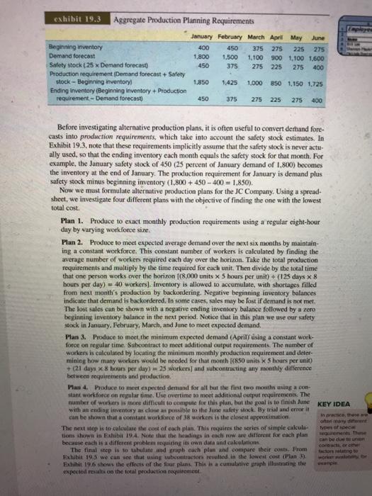

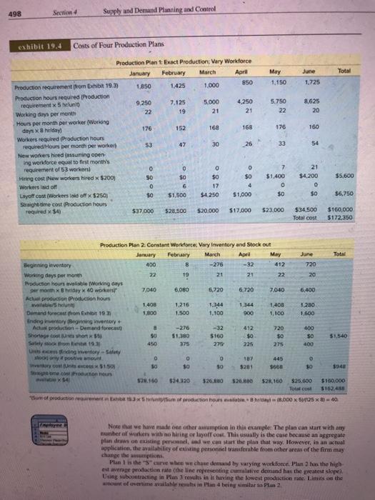
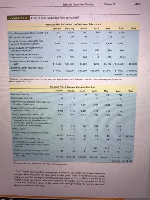
exhibit 19.3 Aggregate Production Planning Requirements January February March April May June Beginning inventory 400 450 375 275 225 275 Demand forecast 1,800 1.500 1.100 900 1.100 1.600 Safety stock (25 x Demand forecast) 450 375 275 225 275 400 Production requirement (Demand forecast Safety stock - Beginning inventory 1,850 1,425 1.000 850 1.150 1.725 Ending inventory (Beginning inventory + Production requirement-Demand forecast 450 375 275 225 275 400 Before investigating alternative production plans, it is often useful to convert derhand fore- casts into production requirements, which take into account the safety stock estimates. In Exhibit 19.3. note that these requirements implicitly assume that the safety stock is never actu. ally used, so that the ending inventory each month equals the safety stock for that month. For example, the January safety stock of 450 (25 percent of January demand of 1.800) becomes the inventory at the end of January. The production requirement for January is demand plus safety stock minus beginning inventory (1.800 + 450 - 400 - 1.850). Now we must formulate alternative production plans for the JC Company. Using a spread sheet, we investigate four different plans with the objective of finding the one with the lowest total cost. Plan 1. Produce to exact monthly production requirements using a regular eight-hour day by varying workforce size Plan 2. Produce to meet expected average demand over the next six months by maintain- ing a constant workforce. This constant number of workers is calculated by finding the average number of workers required each day over the horizon. Take the total production requirements and multiply by the time required for each unit. Then divide by the total time that one person works over the horizon (8,000 units x 5 hours per unit) + (125 days x 8 hours per day) = 40 workers). Inventory is allowed to accumulate, with shortages filled from next month's production by backordering. Negative beginning inventory balances indicate that demand is backordered. In some cases, sales may be lost if demand is not met The lost sales can be shown with a negative ending inventory bulance followed by a zero beginning inventory balance in the next period. Notice that in this plan we use our safety sock in January February March, and June to meet expected demand. Plan 3. Produce to meet the minimum expected demand (Aprily using a constant work- force on regular time. Subcontract to meet additional output requirements. The number of workers is calculated by locating the minimum monthly production requirement and deter mining how many workers would be needed for that month [(850 units x 5 hours per unit) + (21 days x 8 hours per day) = 25 workers and subcontracting any monthly difference between requirements and production Plan 4. Produce to meet expected demand for all but the first two months wing a con stant workforce on regular time. Use overtime to meet additional output requirements. The number of workers is more difficult to compute for this plan, but the goal is to finish June KEY IDEA with an ending inventory as close as possible to the June safety w By trial and errori in chcete can be shown that a constant workforce of 38 workers is the closest approximation on many The next step is to calculate the cost cach plan. This requires the series of simple calcula tions shown in Exhibit 19.4. Note that the headings in each row are different for each plan can be due to because each is a different problem requiring its own data and calculation The final step is to tabulate and graph cach plan and compare their coss. From Exhibit 19. we can see that using subcontractors resulted in the lowest cost (Plan 3). Exhibit 19.6 sl the effects of the four plans. This is a cumulative graph illustrating the expected results on the total production requirement e ape Coro 498 Section 4 Supply and Demand Planning and Control exhibit 19.4 Costs of Four Production Plans Total June 1.725 1,150 5.750 22 8,625 20 176 160 Production Plant Exact Production, Vary Workforce January February March April Production requirement from Exhibit 19.3) 1.850 1.425 850 1,000 Production hours required Production requirement should 9,250 7.125 5.000 4.250 Working days per month 22 19 21 21 Hours per month per worker (Working days 8 heday 176 152 168 168 Workers required Production hours required Hours per month per worken) 30 26 New workers hired (assuming open ing workforce equal to first month's requirement of 63 workers 0 0 0 0 Hiring cost New workers hired x $200) $0 50 $0 Workers laid of 0 6 17 4 Layoff cost Workers told off $250) $0 $1,500 $4.250 $1,000 Straight time cost Production hours required x 54) $37.000 $28.500 $20.000 $17.000 S3 47 33 54 & $5,600 7 $1,400 0 $0 21 $4,200 0 $0 $6,750 $23.000 $34,500 Total cost $160,000 5172.350 400 Production Plan 2. Constant Workforce Vary Inventory and Stock out January February March April May June Total Beginning inventory 8 -276 -32 412 720 Working days per month 22 19 21 21 22 20 Production hours valible Working days per month day X 40 workers 7,040 6,080 6,720 6.720 7.640 6,400 Actus production Production hours www/ht 1.408 1,216 1.344 1,344 1,400 1.280 Dumand forecom EN 1937 1.800 1.500 1.100 900 1,100 1,600 Ending intor Beginning inventory Acum production-Demand forecast -276 -32 412 720 Shortage cost short $0 $1,380 $160 $0 $0 SO $1,540 Sately come 19.3 450 175 275 225 275 400 Uning hvory-Safety Modo Moon 0 0 0 107 445 or counter 5150 so so 5201 5660 $0 $940 mo 28.150 524320 326 NO $26.000 52100 $25.000 $100,000 Total cost 5162416 Burnt of productivement 3x5mtroduction house 8.000 25 - 40 400 Note that we have made one other sumption in this example: The plan can start with any number of one with no hiring or layoff cost. This usually is the case because an agregate plan draws on existing prinel, and we can start the plan that way. However, in an actual application, the availability of existing personnel transferable from other areas of the firm may change the sumption Plan is the cure when we chose demand by varying workforce. Man has the high est average production rate the line representing camlative demand has the greatest slope Using subcontracting in Man results in it having the lowest production rate Limits on the wont of overtime available resus in Plan 4 bing similar to Plan 2 Sales and Operations Planning Chaper 19 499 exhibit 19.4 Costs of Four Production Plans concluded) Total May 1,150 22 June 1.725 20 4.400 4,000 Production Plan 3: Constant Low Workforce Subcontract January February March April Production requirement from Exhibit 193) 1,850 1.425 1.000 850 Working days per month 22 19 21 21 Production hours aveable (Working darys x hriday x 25 workers 4.400 3800 4.200 4,200 Actual production Production hours available the per unit) 880 750 840 Units subcontracted Production requirement - Actual production 665 160 10 Subcontracting cost (Units subcontracted $20) $19.400 $13.300 $3.200 $200 Sitme cost Production hours valablex $41 $17.600 $15,200 516,800 $16,800 840 880 900 970 270 925 $5,400 $18.500 $60,000 $17.600 $16.000 $100,000 $160,000 Total cost TONI 1.338 100 "Minimum production requirement in this example, April s minimum of 50 units. Number of workers required for Aprilis 1850 SV1218 - 25. Productio Plan & Constant Workforce Overtime January February March April May June Beginning inventory 400 0 0 177 554 792 Working days per month 22 19 21 21 22 20 Production hours available (Wowing days 8 tidy H work 6.633 5.776 6384 6.384 6.688 6,080 Regular production Production hours withthat 1.338 1.195 1,277 1.277 1216 Demand forecast hom Eibt 19 1.800 1.500 1.100 1.100 1,500 Units before overeening inoy Reguler she production Demand forces. This number Founded to the neweger --52 -345 554 792 406 Uutine 375 0 0 0 Overtime consta overtime Shox $1.350 $10,350 10 50 SO $0 Solym 193 375 275 225 275 400 Unsessie Bee tycony Dove om 0 0 0 517 or cox5.50 $0 30 1494 5770 $12 Shame on 520.752 21.104 $2,36 520,752 24330 177 $12,210 51:21 5132.000 $165.491 Each of these for plans focused on one particular cos, and the three were simple pure rategies. Obvioudy, there are many other le plans, some of which would use a com bit of workforce dupes, overtime and at the problems at the end of this chapter include examples of such a strategies. In practice, the final plan chosen would come from starting a variety of alternatives and future projections beyond the six-month planning horison we have used