Please help Lab 9

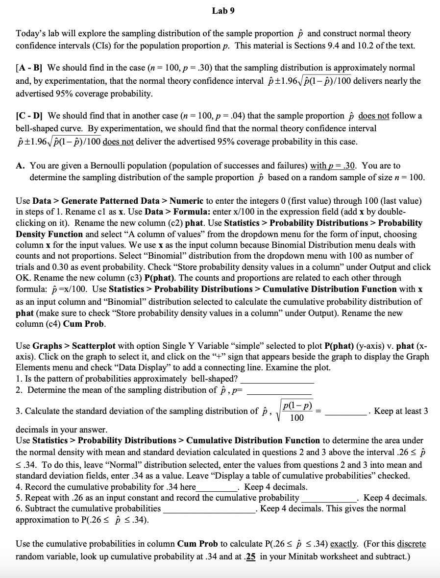
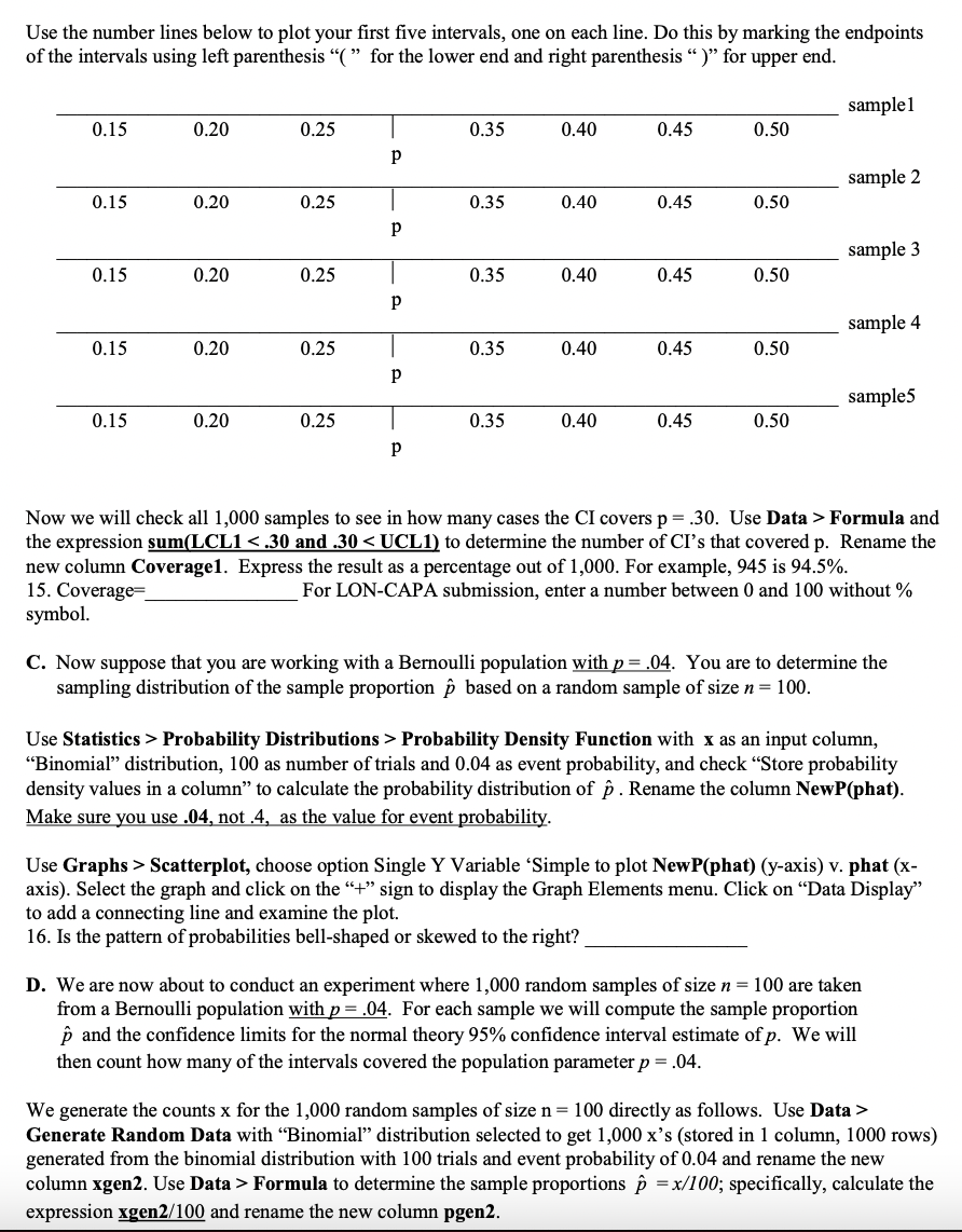
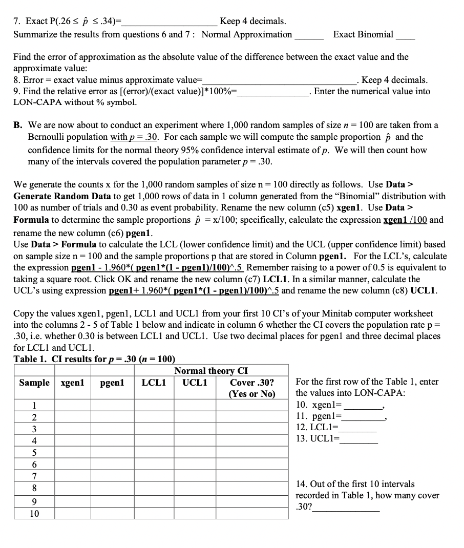
Lab 9 Today's lab will explore the sampling distribution of the sample proportion ,6 and construct normal theory condence intervals (CIs) for the population proportion p. This material is Sections 9.4 and 10.2 of the text. [A - B] We should nd in the case (n = 100, p = .30) that the sampling distribution is approximately normal and, by experimentation, that the normal theory condence interval f3 11961.;I fr)! 100 delivers nearly the advertised 95% coverage probability. [C - D] We should nd that in another case (n = 100, p = .04) that the sample proportion ,6 does not follow a bell-shaped curve. By experimentation, we should nd that the normal theory condence interval 1.\"; i1.961.l'(1 in.\" 100 does not deliver the advertised 95% coverage probability in this case. A. You are given a Bernoulli population (population of successes and failures) with g = .30. You are to determine the sampling distribution of the sample proportion f1 based on a random sample of size n = 100. Use Data 3- Generate Patterned Data 3- Numeric to enter the integers 0 (rst value) through 100 (last value) in steps of 1. Rename c1 as x. Use Data 3* Formula: enter xi 100 in the expression eld (add x by double- clicking on it). Rename the new column (c2) phat. Use Statistics > Probability Distributions 2* Probability D-sity Function and select \"A column of values\" om the dropdown menu for the form of input, choosing colln'nn x for the input values. We use x as the input column because Binomial Distribution menu deals with counts and not proportions. Select \"Binomial\" distribution from the dropdown menu with 100 as number of trials and 0.30 as event probability. Check \"Store probability density values in a column" under Output and click OK. Rename the new column (c3) P(phat). The counts and proportions are related to each other through formula: ,6 =xfl 00. Use Statistics > Probability Distributions 3' Cumulative Distribution Function with x as an input column and \"Binomial\" distribution selected to calculate the cumulative probability distribution of phat (make sure to check \"Store probability density values in a column\" under Output). Rename the new column (c4) Cum Prob. Use Graphs > Scatterplot with option Single Y Variable \"simple\" selected to plot P{phat) (yaxis) v. phat (x- axis). Click on the graph to select it, and click on the \"+\" sign that appears beside the graph to display the Graph Elements menu and check \"Data Display' ' to add a connecting line. Examine the plot. 1. Is the pattern of probabilities approximately bell-shaped? 2. Determine the mean of the sampling distribution of f: , p= N -p) = 100 3. Calculate the standard deviation of the sampling distribution of f1 , . Keep at least 3 decimals in your answer. Use Statistics > Probability Distributions > Cumulative Distribution Function to determine the area under the normal density with mean and standard deviation calculated in questions 2 and 3 above the interval .26 s f) E .34. To do this, leave ' ormal\" distribution selected, enter the values from questions 2 and 3 into mean and standard deviation elds, enter .34 as a value. Leave \"Display a table of cumulative probabilities\" checked. 4. Record the cumulative probability for .34 here . Keep 4 decimals. 5. Repeat with .26 as an input constant and record the cumulative probability . Keep 4 decimals. 6. Subtract the cumulative probabilities . Keep 4 decimals. This gives the normal approximation to P(.26 S f) g .34). Use the cumulative probabilities in column Cum Prob to calculate P(.26 :1 f) i .34) exactly. (For this discrete random variable, look up cmnulative probability at .34 and at g in your Minitab worksheet and subtract.) 7. Exact P(.26 Generate Random Data to get 1,000 rows of data in 1 column generated from the "Binomial" distribution with 100 as number of trials and 0.30 as event probability. Rename the new column (c5) xgenl. Use Data > Formula to determine the sample proportions p = x/100; specifically, calculate the expression xgen1 /100 and rename the new column (c6) pgen1. Use Data > Formula to calculate the LCL (lower confidence limit) and the UCL (upper confidence limit) based on sample size n = 100 and the sample proportions p that are stored in Column pgen1. For the LCL's, calculate the expression pgen1 - 1.960*( pgen1*(1 - pgen1)/100)^.5 Remember raising to a power of 0.5 is equivalent to taking a square root. Click OK and rename the new column (c7) LCL1. In a similar manner, calculate the UCL's using expression pgen1+ 1.960*( pgen*(1 - pgen1)/100)^.5 and rename the new column (c8) UCL1. Copy the values xgenl, pgenl, LCLI and UCLI from your first 10 CI's of your Minitab computer worksheet into the columns 2 - 5 of Table 1 below and indicate in column 6 whether the CI covers the population rate p = 30, i.e. whether 0.30 is between LCL1 and UCL1. Use two decimal places for pgenl and three decimal places for LCL1 and UCL1. Table 1. CI results for p = .30 (n = 100) Normal theory CI Sample xgen1 pgen1 LCL1 UCL1 Cover .30? For the first row of the Table 1, enter (Yes or No) the values into LON-CAPA: 1 10. xgen1= 11. pgenl= 12. LCL1= 13. UCL1= D DO JOVIAWN 14. Out of the first 10 intervals recorded in Table 1, how many cover 30? 10Use the number lines below to plot your rst ve intervals, one on each line. Do this by marking the endpoints of the intervals using left parenthesis \"( \" for the lower end and right parenthesis \" )\" for upper end. sample] 0.15 0.20 0.25 I 0.35 0.40 0.45 0.50 P sample 2 0.15 0.20 0.25 I 0.35 0.40 0.45 0.50 P sample 3 0.15 0.20 0.25 I 0.35 0.40 0.45 0.50 P sample 4 0.15 0.20 0.25 I 0.35 0.40 0.45 0.50 P sampleS 0.15 0.20 0.25 I 0.35 0.40 0.45 0.50 P Now we will check all 1,000 samples to see in how many cases the CI covers p = .30. Use Data > Formula and the expression suml [:CLI Probability Distributions > Probability Density Function with x as an input column, \"Binomial" distribution, 100 as number of trials and 0.04 as event probability, and check \"Store probability density values in a column\" to calculate the probability distribution of ,6 . Rename the column NewPlhat). Make sure you use .04, not .4, as the value for event mbam'lity. Use Graphs > Scatterplot, choose option Single Y Variable 'Simple to plot NewP(phat) (y-axis) v. phat (x- axis). Select the graph and click on the \"+\" sign to display the Graph Elements menu. Click on \"Data Display\" to add a connecting line and examine the plot. 16. Is the pattern of probabilities bell-shaped or skewed to the right? D. We are now about to conduct an experiment where 1,000 random samples of size n = 100 are taken from a Bernoulli population with p = .04. For each sample we will compute the sample proportion ,6 and the condence limits for the normal theory 95% condence interval estimate of p. We will then count how many of the intervals covered the population parameter p = .04. We generate the counts x for the 1,000 random samples of size n = 100 directly as follows. Use Data > Generate Random Data with \"Binomial\" distribution selected to get 1,000 x's (stored in 1 column, 1000 rows) generated from the binomial distribution with 100 trials and event probability of 0.04 and rename the new column xgenl. Use Data =- Formula to determine the sample proportions 13 = #100; specically, calculate the expression xgenz.' 100 and rename the new column pgenz. Use Data > Formula to calculate the LCL and the UCL based on sample size n = 100 and the sample proportions p that are stored in Column pgen2. For LCL, calculate the expression pgen2 - 1.960*( pgen2*(1 =pgen2)/100)4.5 and rename the new column LCL2. In a similar manner, calculate the UCL's using expression pgen2 + 1.960*( pgen2*(1 - pgen2)/100)^.5 and rename UCL2. Copy the values xgen2, pgen2, LCL2 and UCL2 from your first 10 CI's of your MTB computer worksheet into columns 2 - 5 of Table 2 below and indicate in column 6 whether the CI covers the population rate p = .04. (Use two decimal places for pgen2 and three decimal places for LCL2 and UCL2.) Table 2. CI results for p = .04 (n = 100) Normal theory CI Sample xgen2 pgen2 LCL2 UCL2 Cover .04? For the first row of Table 2, enter the (Yes or No) values as responses to questions 17 and 18: 17. xgen2= 18. pgen2= DOO JON UI A WINE 19. Out of the first 10 intervals recorded in Table 2, how many cover .04?_ 10 Now we will check all 1,000 samples to see in how many cases the CI covers p = .04. Use Data > Formula and the statement sum(LCL2