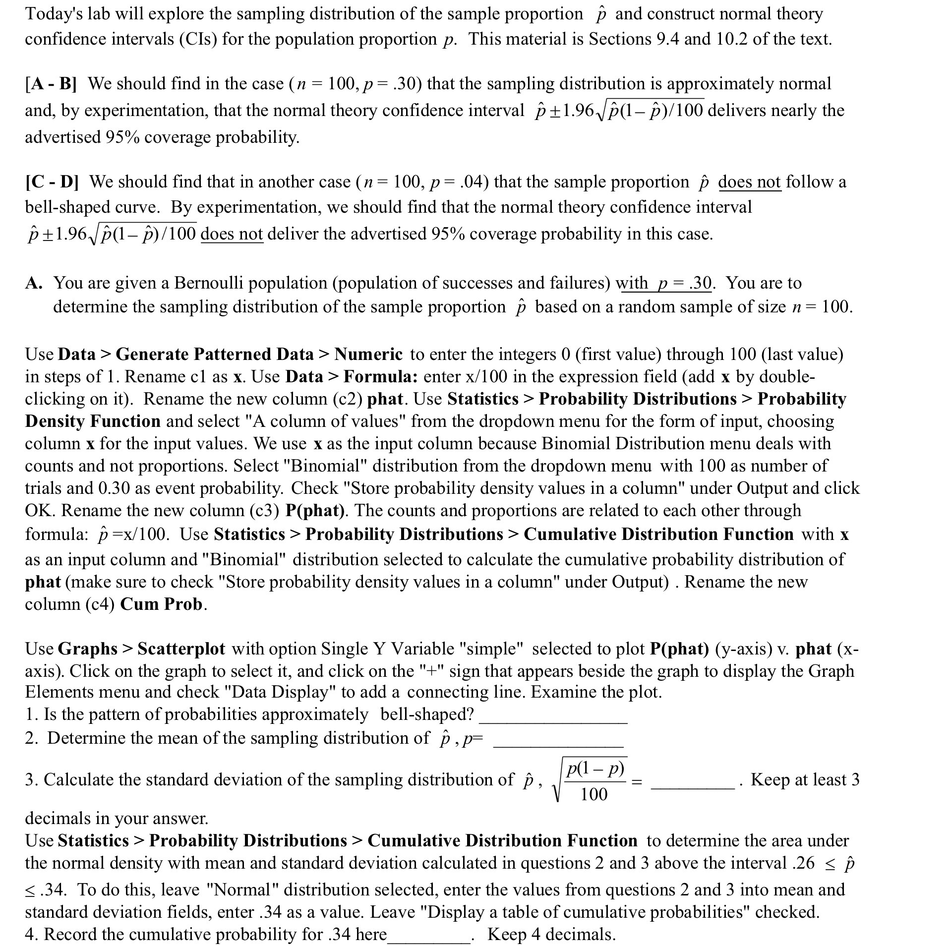
Today's lab Will explore the sampling distribution of the sample proportion f) and construct normal theory confidence intervals (CIs) for the population proportion p. This material is Sections 9.4 and 10.2 of the text. [A - B] We should find in the case (n = 100, p = .30) that the sampling distribution is approximately normal and, by experimentation, that the normal theory condence interval 13 i 1.961/f3(l )/ 100 delivers nearly the advertised 95% coverage probability. [C D] We should find that in another case (n = 100, p = .04) that the sample proportion [7 does not follow a bell- shaped curve. By experimentation, we should find that the normal theory condence interval 13 i 1.96.1360 )/ 100 does not deliver the advertised 95% coverage probability in this case. A. You are given a Bernoulli population (population of successes and failures) with Q = .30. You are to determine the sampling distribution of the sample proportion f9 based on a random sample of size n = 100. Use Data > Generate Patterned Data > Numeric to enter the integers 0 (first value) through 100 (last value) in steps of 1. Rename cl as X. Use Data > Formula: enter x/l 00 in the expression field (add x by double- clicking on it). Rename the new column (c2) phat. Use Statistics > Probability Distributions > Probability Density Function and select "A column of values" from the dropdown menu for the form of input, choosing column x for the input values. We use X as the input column because Binomial Distribution menu deals with counts and not proportions. Select "Binomial" distribution from the dropdown menu with 100 as number of trials and 0.30 as event probability. Check "Store probability density values in a column" under Output and click OK. Rename the new column (c3) P(phat). The counts and proportions are related to each other through formula: {9 =x/ 100. Use Statistics > Probability Distributions > Cumulative Distribution Function with x as an input column and "Binomial" distribution selected to calculate the cumulative probability distribution of phat (make sure to check "Store probability density values in a column" under Output) . Rename the new column (c4) Cum Prob. Use Graphs > Scatterplot With option Single Y Variable "simple" selected to plot P(phat) (yaxis) v. phat (x- axis). Click on the graph to select it, and click on the "+" sign that appears beside the graph to display the Graph Elements menu and check "Data Display" to add a connecting line. Examine the plot. 1. Is the pattern of probabilities approximately bell-shaped? 2. Determine the mean of the sampling distribution of f) , p: 3. Calculate the standard deviation of the sampling distribution of f9 , "D (110010) = . Keep at least 3 decimals in your answer. Use Statistics > Probability Distributions > Cumulative Distribution Function to determine the area under the normal density with mean and standard deviation calculated in questions 2 and 3 above the interval .26 g f) g .34. To do this, leave "Normal" distribution selected, enter the values from questions 2 and 3 into mean and standard deviation elds, enter .34 as a value. Leave "Display a table of cumulative probabilities" checked. 4. Record the cumulative probability for .34 here . Keep 4 decimals