Please help me find the error in my formulas, NOT solve, it says they are incorrect. Thank you!!

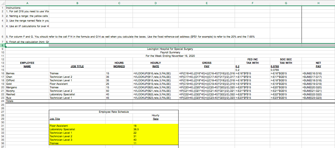
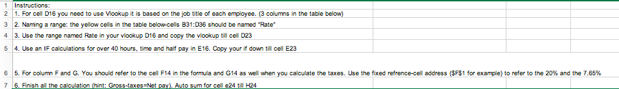
A B D E F H 1 Instructions: 2 1. For cell D16 you need to use Vio 3 2. Naming a range: the yellow cells 4 3. Use the range named Rate in you 5 4. Use an IF calculations for over 4 NET PAY 6 5. For column F and G. You should refer to the cell F14 in the formula and G14 as well when you calculate the taxes. Use the fixed refrence-cell address ($F$1 for example) to refer to the 20% and the 7.65% 7 6. Finish all the calculation hint: Gr 8 9 Lexington Hospital for Special Surgery 10 Payroll Summary 11 For the Week Ending November 16, 2020 12 FED INC 13 EMPLOYEE HOURS HOURLY GROSS TAX WITH 14 NAME JOB TITLE WORKED RATE PAY 0.2 15 0.2 16 Barnes Trainee 15 =VLOOKUP(B16,rate,3,FALSE) =IF(C16~40.((D1640)+((C16-407"D16)72),D16 --E16'$F$15 17 Chen Technician Level 2 35 =VLOOKUP(B17.rate,3,FALSE) =IF(C1740.((D17*40)+(((C17-40)*D17)y2),D17 =-E17"$F$15 18 Clifford Technician Level 1 35 =VLOOKUP(B18.rate.3. FALSE =IF(C18>40.((D18*40)+{{{C18-40)*D18)72).D18 --E18*$F$15 19 Gold Floor Assistant 25 =VLOOKUP(B19, rate,3,FALSE) =IF(C1940.((D19*40)+{{C19-40y"D19)/2).D19 --E19*$F$15 20 Mangano Trainee 15 =VLOOKUP(B20 rate,3,FALSE) =IF(C20~40.((D20-40)+(((C20-40) D20)72), D20 --E20 $F$15 21 Murphy Technician Level 2 50 =VLOOKUP(B21.rate,3,FALSE) =IF(C21>40.((D21*40)+(((C21-40)*D21)2), D21 --E21"$F$15 22 Rashad Laboratory Specialist 40 =VLOOKUP(B22 rate, 3,FALSE) =IF(C2240.((D22-40)+{{{C22-40) D22)2), D22 --E22"$F$15 23 Ruiz Technician Level 1 45 =VLOOKUP(B23,rate,3,FALSE) =1F(C23>40.{{D23-40)+{{(C23-40)*D23)/2),D23 --E23*$F$15 24 Totals 25 26 27 Employee Rate Schedule 28 Hourly 29 Job Title Rate 30 31 Floor Assistant 18 32 Laboratory Specialist 38.5 33 Technician Level 1 22 34 Technician Level 2 31 35 Technician Level 3 40 36 Trainee 11 37 SOC SEC TAX WITH 0.0765 0.0765 --E16*$G$15 --E17"$G$15 --E18*$G$15 --E19"$G$15 --E20-$G$15 --E21"$G$15 --E22*$G$15 --E23"$G$15 =SUME 16:16) =SUME 17:17) ESUME 18:G18) =SUME 19:G19) =SUME20:G20) =SUM(E21:G21) ESUME22:G22) =SUME23:G23) 1 Instructions: 2 1. For cell D16 you need to use Vlookup it is based on the job title of each employee. (3 columns in the table below) 3 2. Naming a range: the yellow cells in the table below-cells B31:036 should be named "Rate" 4 3. Use the range named Rate in your vlookup D16 and copy the vlookup till cell D23 5 4. Use an IF calculations for over 40 hours, time and half pay in E16. Copy your if down till cell E23 6 5. For column F and G. You should refer to the cell F14 in the formula and G14 as well when you calculate the taxes. Use the fixed refrence-cell address ($F$1 for example) to refer to the 20% and the 7.65% 7 6. Finish all the calculation (hint: Gross-taxes=Net pay). Auto sum for cell e24 till H24 A B D E F H 1 Instructions: 2 1. For cell D16 you need to use Vio 3 2. Naming a range: the yellow cells 4 3. Use the range named Rate in you 5 4. Use an IF calculations for over 4 NET PAY 6 5. For column F and G. You should refer to the cell F14 in the formula and G14 as well when you calculate the taxes. Use the fixed refrence-cell address ($F$1 for example) to refer to the 20% and the 7.65% 7 6. Finish all the calculation hint: Gr 8 9 Lexington Hospital for Special Surgery 10 Payroll Summary 11 For the Week Ending November 16, 2020 12 FED INC 13 EMPLOYEE HOURS HOURLY GROSS TAX WITH 14 NAME JOB TITLE WORKED RATE PAY 0.2 15 0.2 16 Barnes Trainee 15 =VLOOKUP(B16,rate,3,FALSE) =IF(C16~40.((D1640)+((C16-407"D16)72),D16 --E16'$F$15 17 Chen Technician Level 2 35 =VLOOKUP(B17.rate,3,FALSE) =IF(C1740.((D17*40)+(((C17-40)*D17)y2),D17 =-E17"$F$15 18 Clifford Technician Level 1 35 =VLOOKUP(B18.rate.3. FALSE =IF(C18>40.((D18*40)+{{{C18-40)*D18)72).D18 --E18*$F$15 19 Gold Floor Assistant 25 =VLOOKUP(B19, rate,3,FALSE) =IF(C1940.((D19*40)+{{C19-40y"D19)/2).D19 --E19*$F$15 20 Mangano Trainee 15 =VLOOKUP(B20 rate,3,FALSE) =IF(C20~40.((D20-40)+(((C20-40) D20)72), D20 --E20 $F$15 21 Murphy Technician Level 2 50 =VLOOKUP(B21.rate,3,FALSE) =IF(C21>40.((D21*40)+(((C21-40)*D21)2), D21 --E21"$F$15 22 Rashad Laboratory Specialist 40 =VLOOKUP(B22 rate, 3,FALSE) =IF(C2240.((D22-40)+{{{C22-40) D22)2), D22 --E22"$F$15 23 Ruiz Technician Level 1 45 =VLOOKUP(B23,rate,3,FALSE) =1F(C23>40.{{D23-40)+{{(C23-40)*D23)/2),D23 --E23*$F$15 24 Totals 25 26 27 Employee Rate Schedule 28 Hourly 29 Job Title Rate 30 31 Floor Assistant 18 32 Laboratory Specialist 38.5 33 Technician Level 1 22 34 Technician Level 2 31 35 Technician Level 3 40 36 Trainee 11 37 SOC SEC TAX WITH 0.0765 0.0765 --E16*$G$15 --E17"$G$15 --E18*$G$15 --E19"$G$15 --E20-$G$15 --E21"$G$15 --E22*$G$15 --E23"$G$15 =SUME 16:16) =SUME 17:17) ESUME 18:G18) =SUME 19:G19) =SUME20:G20) =SUM(E21:G21) ESUME22:G22) =SUME23:G23) 1 Instructions: 2 1. For cell D16 you need to use Vlookup it is based on the job title of each employee. (3 columns in the table below) 3 2. Naming a range: the yellow cells in the table below-cells B31:036 should be named "Rate" 4 3. Use the range named Rate in your vlookup D16 and copy the vlookup till cell D23 5 4. Use an IF calculations for over 40 hours, time and half pay in E16. Copy your if down till cell E23 6 5. For column F and G. You should refer to the cell F14 in the formula and G14 as well when you calculate the taxes. Use the fixed refrence-cell address ($F$1 for example) to refer to the 20% and the 7.65% 7 6. Finish all the calculation (hint: Gross-taxes=Net pay). Auto sum for cell e24 till H24