Please help me to rebulid the codes to fix the error of "'NoneType' object is not callable" for both LQR and MPC, and help me to check and rewrite the wrong part as I can not output the figure shown as an example as follows:

The codes are:

import numpy as np import cvxpy as cp   def Setup_Derivative(param):    ## this function is optional     ## TODO     return None # TODO   def Fun_Jac_dt(x, u, param):     L_f = param["L_r"]    L_r = param["L_f"]    h = param["h"]     psi = x[2]    v   = x[3]    delta = u[0]    a   = u[1]     A = np.zeros((4, 4))    B = np.zeros((4, 2))      A[0, 0] = 1    A[0, 2] = -h*v*np.sin(psi+np.arctan((L_r*np.arctan(delta))/(L_f+L_r)))    A[0, 3] = h*np.cos(psi+np.arctan((L_r*np.arctan(delta))/(L_f+L_r)))     A[1, 1] = 1    A[1, 2] = -h*v*np.cos(psi+np.arctan((L_r*np.arctan(delta))/(L_f+L_r)))    A[1, 3] = h*np.sin(psi+np.arctan((L_r*np.arctan(delta))/(L_f+L_r)))       A[2, 2] = 1    A[2, 3] = (h*np.arctan(delta)/(((L_r**2*delta**np.arctan(delta)**2)/(L_f+L_r)**2 + 1)**(1/2)*(L_f+L_r)))    A[3, 3] = 1     B[0, 1] = -(h*L_r*v*np.sin(psi+np.arctan((L_r*np.arctan(delta))/(L_f+L_r))))/((delta**2 + 1)*((L_r**2*np.arctan(delta)**2)/(L_f+L_r)**2+1)*(L_f+L_r))    B[1, 1] = (h*L_r*v*np.cos(psi+np.arctan((L_r*np.arctan(delta))/(L_f+L_r))))/((delta**2 + 1)*((L_r**2*np.arctan(delta)**2)/(L_f+L_r)**2+1)*(L_f+L_r))    B[2, 1] = (h*v)/((delta**2 + 1)*((L_r**2*np.arctan(delta)**2)/(L_f+L_r)**2+1)**(3/2)*(L_f+L_r))    B[3, 0] = h     return [A, B] def Student_Controller_LQR(x_bar, u_bar, x0, Fun_Jac_dt, param):         dim_state = x_bar.shape[1]    dim_ctrl  = u_bar.shape[1]     n_u = u_bar.shape[0] * u_bar.shape[1]    n_x = x_bar.shape[0] * x_bar.shape[1]    n_var = n_u + n_x     n_eq = x_bar.shape[1] * u_bar.shape[0]    n_ieq = u_bar.shape[1] * u_bar.shape[0]     # Define the parameters    Q = np.eye(4)     Q[0, 0] = 10000    Q[3, 3] = 10000    Q[1, 1] = 200000    Q[2, 2] = 10000    R = np.eye(2)    R[0, 0] = 9000    R[1, 1] = 7000    Pt = np.eye(4) * 10000    Pt = np.eye(4) * 10       #Define the cost function    np.random.seed(1)    P = np.zeros((n_var, n_var))     for k in range(u_bar.shape[0]):        P[k * x_bar.shape[1]:(k+1) * x_bar.shape[1], k * x_bar.shape[1]:(k+1) * x_bar.shape[1]] = Q        P[n_x + k * u_bar.shape[1]:n_x + (k+1) * u_bar.shape[1], n_x + k * u_bar.shape[1]:n_x + (k+1) * u_bar.shape[1]] = R     P[n_x - x_bar.shape[1]:n_x, n_x - x_bar.shape[1]:n_x] = Pt    P = (P + P.T) / 2    q = np.zeros((n_var, 1))     # Define the constraints    A = np.zeros((n_eq, n_var))    b = np.zeros(n_eq)     G = np.zeros((n_ieq, n_var))    ub = np.zeros(n_ieq)    lb = np.zeros(n_ieq)     u_lb = param["delta_lim"]    u_ub = param["a_lim"]     for k in range(u_bar.shape[0]):        AB = Fun_Jac_dt(x_bar[k,:], u_bar[k,:], param)        A[k*dim_state:(k+1)*dim_state, dim_state:(k+1)*dim_state] = AB[0]        A[k*dim_state:(k+1)*dim_state, (k+1)*dim_state:(k+2)*dim_state] = -np.eye(dim_state)        A[k*dim_state:(k+1)*dim_state, n_x + k*dim_ctrl:n_x + (k+1)*dim_ctrl] = AB[1]         G[k*dim_ctrl:(k+1)*dim_ctrl, n_x + k*dim_ctrl:n_x + (k+1)*dim_ctrl] = np.eye(dim_ctrl)        ub[k*dim_ctrl:(k+1)*dim_ctrl] = u_ub - u_bar[k,:]        lb[k*dim_ctrl:(k+1)*dim_ctrl] = u_lb - u_bar[k,:]                # Define and solve the CVXPY problem    x = cp.Variable(n_var)     cons = [A @ x == b, x[0:dim_state] == x0 - x_bar[0, :]]     prob = cp.Problem(cp.Minimize((1/2)*cp.quad_form(x, P) + q.T @ x), cons)     prob.solve(verbose=False, max_iter = 10000)     return (x.value[n_x:n_x + dim_ctrl] + u_bar[0, :])   def Student_Controller_CMPC(x_bar, u_bar, x0, Fun_Jac_dt, param):       dim_state = u_bar.shape[1]    dim_ctrl  = x_bar.shape[1]     n_u = u_bar.shape[0] * u_bar.shape[1]    n_x = x_bar.shape[0] * x_bar.shape[1]    n_var = n_u + n_x     n_eq = x_bar.shape[0] * u_bar.shape[1]    n_ieq = u_bar.shape[1] * x_bar.shape[1]   # Define the parameters    Pt = np.eye(4) * 700    Q = np.eye(4) * 100    R = np.eye(2) * 200000   # Define the cost funcgion     np.random.seed(1)    P = np.zeros((n_var, n_var))     for k in range(u_bar.shape[0]):        P[k * x_bar.shape[1]:(k+1) * x_bar.shape[1], k * x_bar.shape[1]:(k+1) * x_bar.shape[1]] = Q        P[n_x + k * u_bar.shape[1]:n_x + (k+1) * u_bar.shape[1], n_x + k * u_bar.shape[1]:n_x + (k+1) * u_bar.shape[1]] = R     P[n_x - x_bar.shape[1]:n_x, n_x - x_bar.shape[1]:n_x] = Pt    P = (P + P.T) / 2    q = np.zeros((n_var, 1))     # Define the constraints    A = np.zeros((n_eq, n_var))    b = np.zeros(n_eq)     G = np.zeros((n_ieq, n_var))    ub = np.zeros(n_ieq)    lb = np.zeros(n_ieq)     u_lb = param["delta_lim"]    u_ub = param["a_lim"]     for k in range(u_bar.shape[0]):        AB = Fun_Jac_dt(x_bar[k,:], u_bar[k,:], param)        A[k*dim_state:(k+1)*dim_state, dim_state:(k+1)*dim_state] = AB[0]        A[k*dim_state:(k+1)*dim_state, (k+1)*dim_state:(k+2)*dim_state] = -np.eye(dim_state)        A[k*dim_state:(k+1)*dim_state, n_x + k*dim_ctrl:n_x + (k+1)*dim_ctrl] = AB[1]         G[k*dim_ctrl:(k+1)*dim_ctrl, n_x + k*dim_ctrl:n_x + (k+1)*dim_ctrl] = np.eye(dim_ctrl)        ub[k*dim_ctrl:(k+1)*dim_ctrl] = u_ub - u_bar[k,:]        lb[k*dim_ctrl:(k+1)*dim_ctrl] = u_lb - u_bar[k,:]     # Define and solve the CVXPY problem.    x = cp.Variable(n_var)    cons = [G @ x 

And the requirements are:

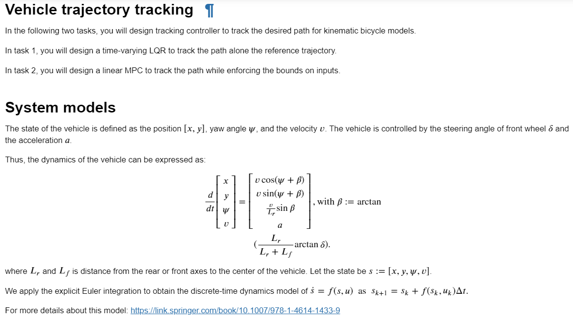
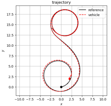
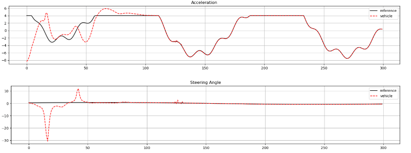
Vehicle trajectory tracking 1 In the following two tasks, you will design tracking controller to track the desired path for kinematic bicycle models. In task 1, you will design a time-varying LQR to track the path alone the reference trajectory. In task 2, you will design a linear MPC to track the path while enforcing the bounds on inputs. System models The state of the vehicle is defined as the position [x, y], yaw angle y, and the velocity v. The vehicle is controlled by the steering angle of front wheel & and the acceleration a. Thus, the dynamics of the vehicle can be expressed as: v cos(y + p) v sin(y + B) F- sin p a Lr Lp + L f where L, and Lf is distance from the rear or front axes to the center of the vehicle. Let the state be s := [x, y, w, v]. We apply the explicit Euler integration to obtain the discrete-time dynamics model of s = f(s, u) as Sk+1 = $k + f(sk, Uk)At. For more details about this model: https://link.springer.com/book/10.1007/978-1-4614-1433-9 d dt X y Y , with := arctan -arctan 8).