Please help me with my M/G/2 queueing system spreadsheet simulation question. Random numbers can be found accordingly for type1, 2 and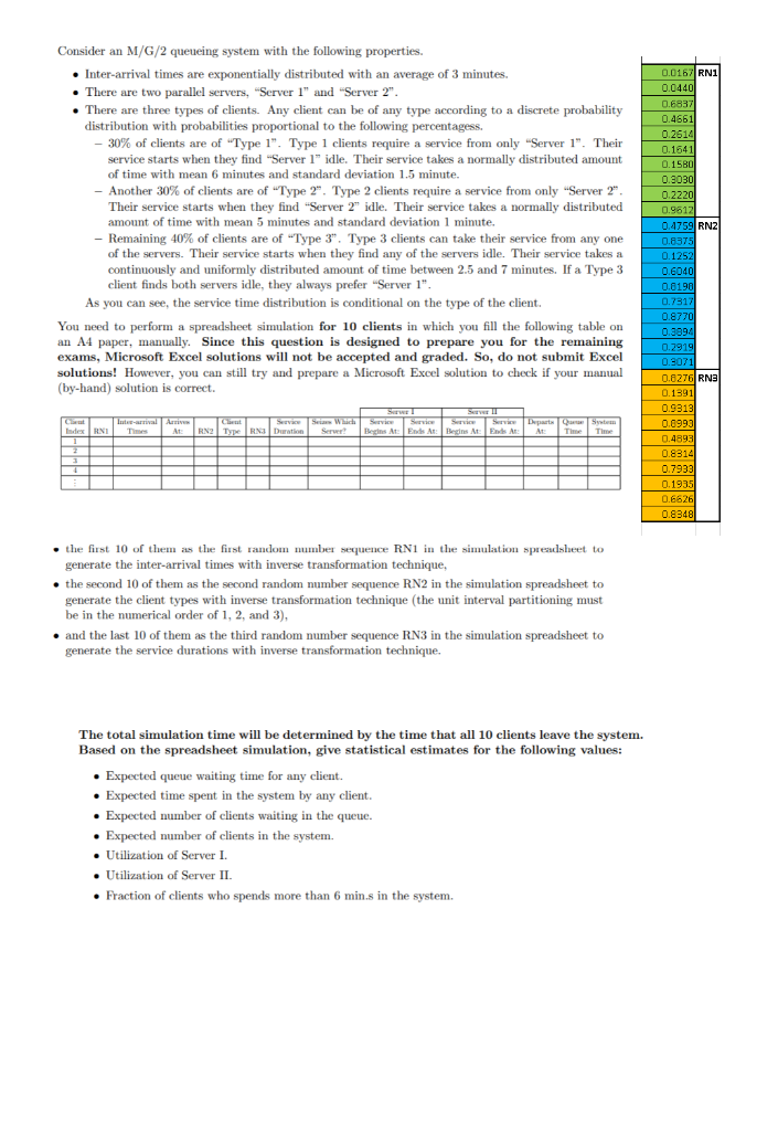

Consider an M/G/2 queueing system with the following properties. Inter-arrival times are exponentially distributed with an average of 3 minutes. . There are two parallel servers. "Server 1" and "Server 2". There are three types of clients. Any client can be of any type according to a discrete probability distribution with probabilities proportional to the following percentagess. 30% of clients are of "Type 1". Type 1 clients require a service from only Server 1". Their service starts when they find "Server 1" idle. Their service takes a normally distributed amount of time with mean 6 minutes and standard deviation 1.5 minute. Another 30% of clients are of "Type 2". Type 2 clients require a service from only "Server 2". Their service starts when they find "Server 2" idle. Their service takes a normally distributed amount of time with mean 5 minutes and standard deviation 1 minute. Remaining 40% of clients are of "Type 3". Type 3 clients can take their service from any one of the servers. Their service starts when they find any of the servers idle. Their service takes a continuously and uniformly distributed amount of time between 2.5 and 7 minutes. If a Type 3 client finds both servers idle, they always prefer "Server 1". As you can see, the service time distribution is conditional on the type of the client. You need to perform a spreadsheet simulation for 10 clients in which you fill the following table on an A4 paper, manually. Since this question is designed to prepare you for the remaining exams, Microsoft Excel solutions will not be accepted and graded. So, do not submit Excel solutions! However, you can still try and prepare a Microsoft Excel solution to check if your manual (by-hand) solution is correct. Sw Server Interval Arrive Service Service Departamente RNZ Type RNB Duration 0.0167 RN1 0.0440 0.6837 0.4661 0.26141 0.1541 0.1580 0.3030 0.2220 0.9612 0.4759 RNZI 0.8375 0.1252 0.6040 0.6190 0.7317 0.8770 0.3894 0.29191 0.3071 0.8276 RNS 0.1991 0.9313 0.6993 0.4893 0.8314 0.7933 0.1935 0.6626 0.8348 Service IndexRNI Times At Serwet Begins At: Eten Es At At Time Time the first 10 of them as the first random number sequence RN1 in the simulation spreadsheet to generate the inter-arrival times with inverse transformation technique, the second 10 of them as the second random number sequence RN2 in the simulation spreadsheet to generate the client types with inverse transformation technique (the unit interval partitioning must be in the numerical order of 1, 2, and 3), . and the last 10 of them as the third random number sequence RN3 in the simulation spreadsheet to generate the service durations with inverse transformation technique. The total simulation time will be determined by the time that all 10 clients leave the system. Based on the spreadsheet simulation, give statistical estimates for the following values: Expected queue waiting time for any client. Expected time spent in the system by any client. Expected number of clients waiting in the queue. Expected number of clients in the system. Utilization of Server I. . Utilization of Server II. Fraction of clients who spends more than 6 min.s in the system. Consider an M/G/2 queueing system with the following properties. Inter-arrival times are exponentially distributed with an average of 3 minutes. . There are two parallel servers. "Server 1" and "Server 2". There are three types of clients. Any client can be of any type according to a discrete probability distribution with probabilities proportional to the following percentagess. 30% of clients are of "Type 1". Type 1 clients require a service from only Server 1". Their service starts when they find "Server 1" idle. Their service takes a normally distributed amount of time with mean 6 minutes and standard deviation 1.5 minute. Another 30% of clients are of "Type 2". Type 2 clients require a service from only "Server 2". Their service starts when they find "Server 2" idle. Their service takes a normally distributed amount of time with mean 5 minutes and standard deviation 1 minute. Remaining 40% of clients are of "Type 3". Type 3 clients can take their service from any one of the servers. Their service starts when they find any of the servers idle. Their service takes a continuously and uniformly distributed amount of time between 2.5 and 7 minutes. If a Type 3 client finds both servers idle, they always prefer "Server 1". As you can see, the service time distribution is conditional on the type of the client. You need to perform a spreadsheet simulation for 10 clients in which you fill the following table on an A4 paper, manually. Since this question is designed to prepare you for the remaining exams, Microsoft Excel solutions will not be accepted and graded. So, do not submit Excel solutions! However, you can still try and prepare a Microsoft Excel solution to check if your manual (by-hand) solution is correct. Sw Server Interval Arrive Service Service Departamente RNZ Type RNB Duration 0.0167 RN1 0.0440 0.6837 0.4661 0.26141 0.1541 0.1580 0.3030 0.2220 0.9612 0.4759 RNZI 0.8375 0.1252 0.6040 0.6190 0.7317 0.8770 0.3894 0.29191 0.3071 0.8276 RNS 0.1991 0.9313 0.6993 0.4893 0.8314 0.7933 0.1935 0.6626 0.8348 Service IndexRNI Times At Serwet Begins At: Eten Es At At Time Time the first 10 of them as the first random number sequence RN1 in the simulation spreadsheet to generate the inter-arrival times with inverse transformation technique, the second 10 of them as the second random number sequence RN2 in the simulation spreadsheet to generate the client types with inverse transformation technique (the unit interval partitioning must be in the numerical order of 1, 2, and 3), . and the last 10 of them as the third random number sequence RN3 in the simulation spreadsheet to generate the service durations with inverse transformation technique. The total simulation time will be determined by the time that all 10 clients leave the system. Based on the spreadsheet simulation, give statistical estimates for the following values: Expected queue waiting time for any client. Expected time spent in the system by any client. Expected number of clients waiting in the queue. Expected number of clients in the system. Utilization of Server I. . Utilization of Server II. Fraction of clients who spends more than 6 min.s in the system