Please help solve this question.

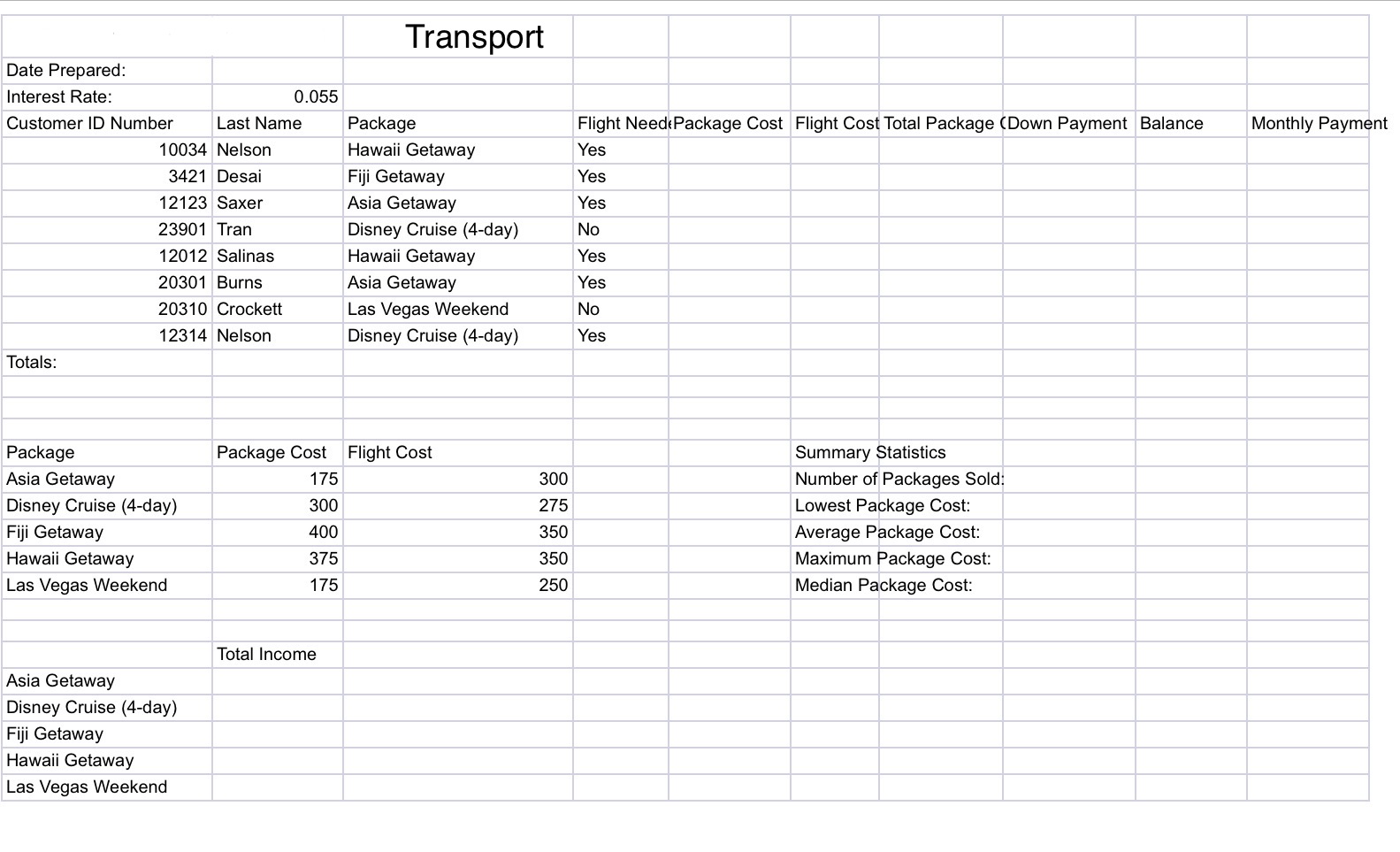
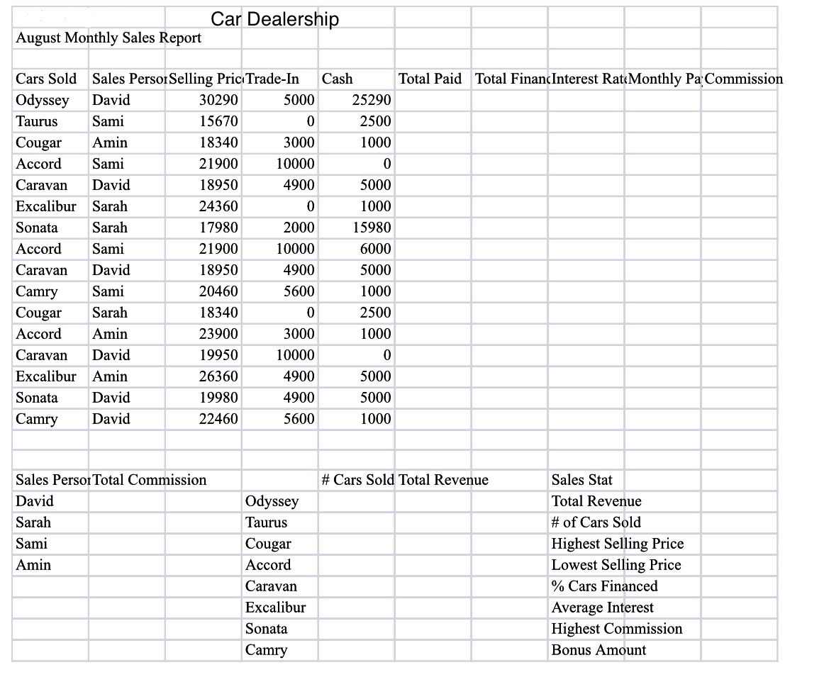
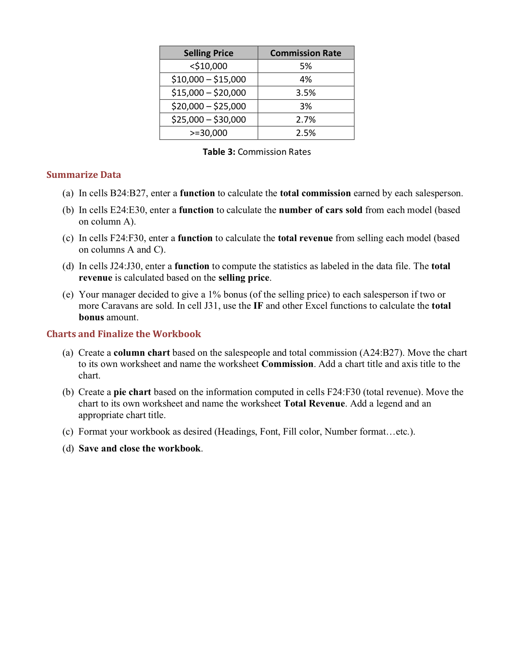
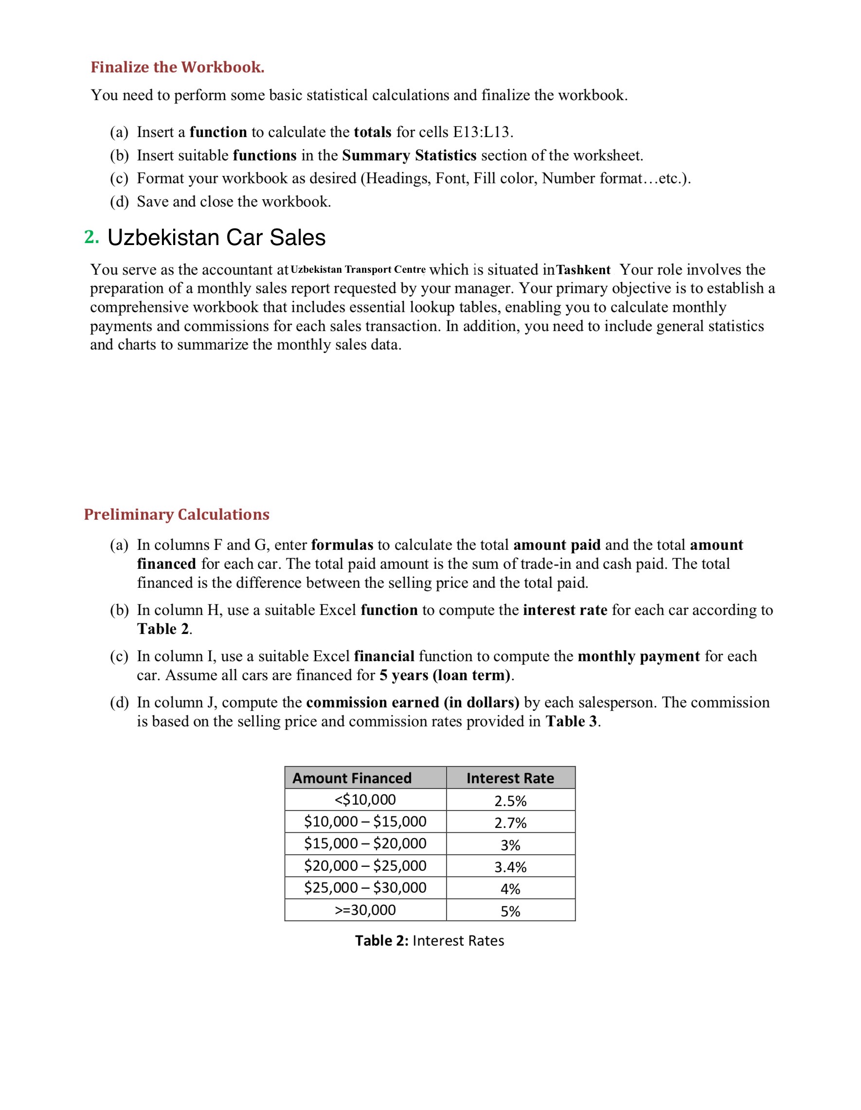
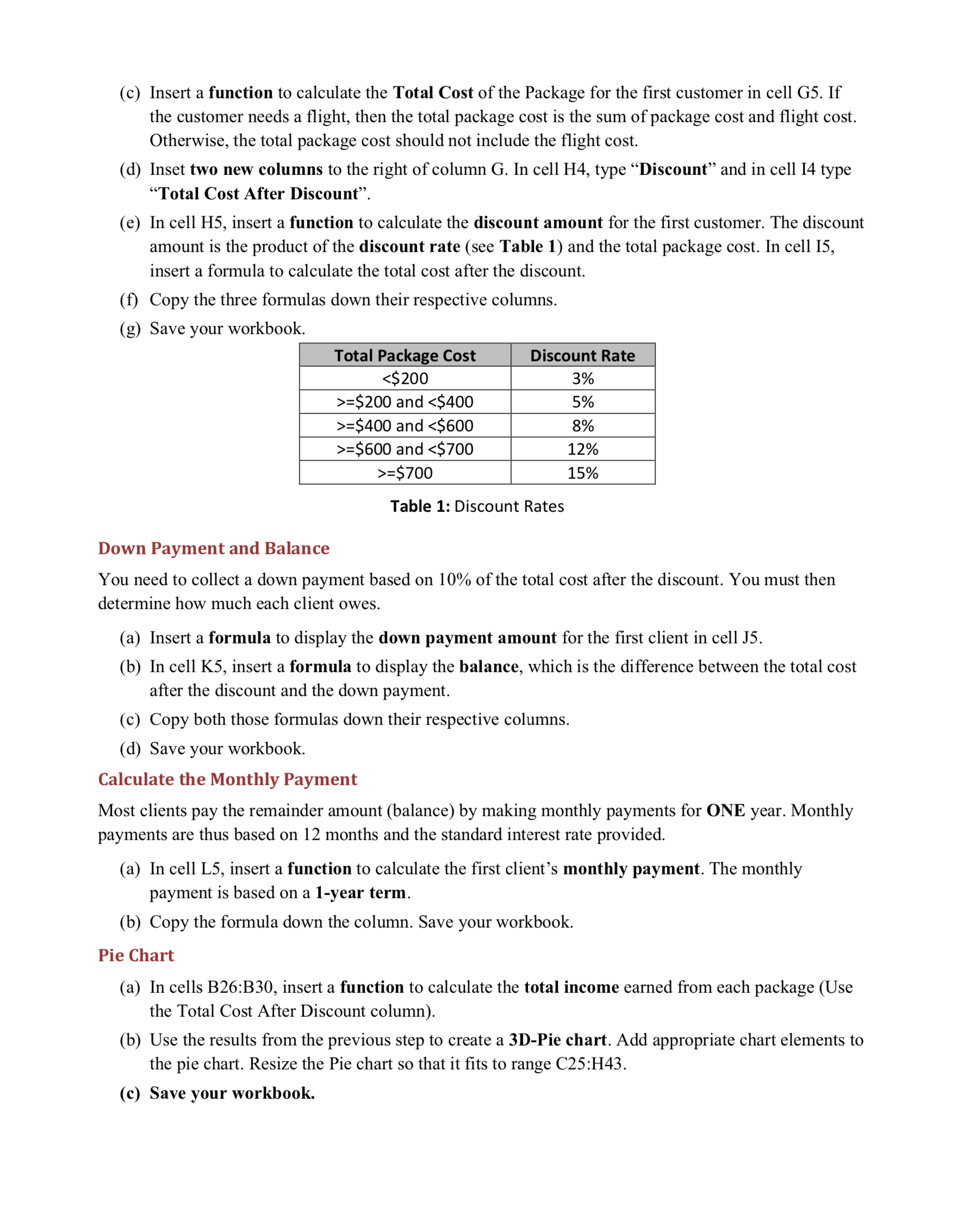
Table 3: Commission Rates Summarize Data (a) In cells B24:B27, enter a function to calculate the total commission earned by each salesperson. (b) In cells E24:E30, enter a function to calculate the number of cars sold from each model (based on column A). (c) In cells F24:F30, enter a function to calculate the total revenue from selling each model (based on columns A and C). (d) In cells J24:J30, enter a function to compute the statistics as labeled in the data file. The total revenue is calculated based on the selling price. (e) Your manager decided to give a 1\% bonus (of the selling price) to each salesperson if two or more Caravans are sold. In cell J31, use the IF and other Excel functions to calculate the total bonus amount. Charts and Finalize the Workbook (a) Create a column chart based on the salespeople and total commission (A24:B27). Move the chart to its own worksheet and name the worksheet Commission. Add a chart title and axis title to the chart. (b) Create a pie chart based on the information computed in cells F24:F30 (total revenue). Move the chart to its own worksheet and name the worksheet Total Revenue. Add a legend and an appropriate chart title. (c) Format your workbook as desired (Headings, Font, Fill color, Number format...etc.). (d) Save and close the workbook. 1. Uzbekistan Transport Centre You work as an agent at Uzbekistan Transport Centre, where your primary responsibility is to monitor and manage end-of-summer sales promotions. These promotions offer customers the flexibility to purchase vacation packages with or without airfare. As part of your role, you must gather an initial down payment amounting to 10% of the package's total cost. A significant portion of your clientele opts for a convenient monthly payment plan spanning one year, and you calculate these payments using the interest rate amount provided in the startup file. Furthermore, you are tasked with generating comprehensive statistical reports to present to your manager. It's essential to periodically validate your calculations and formulas through spot-checks to ensure accuracy and reliability. Calculate Costs and Discounts You are ready to calculate the total costs. The total cost is determined based on each customer's package type, using the lookup table. (a) In cell E5, insert a function to display the package cost for the first customer, based on the Package. The cost lookup table is in A18:C22. (b) In cell F5, insert a function to display the Flight Cost for the first customer, based on the Package. The cost lookup table is in A18:C22. Finalize the Workbook. You need to perform some basic statistical calculations and finalize the workbook. (a) Insert a function to calculate the totals for cells E13:L13. (b) Insert suitable functions in the Summary Statistics section of the worksheet. (c) Format your workbook as desired (Headings, Font, Fill color, Number format...etc.). (d) Save and close the workbook. 2. Uzbekistan Car Sales You serve as the accountant at Uzbekistan Transport Centre which is situated inTashkent Your role involves the preparation of a monthly sales report requested by your manager. Your primary objective is to establish a comprehensive workbook that includes essential lookup tables, enabling you to calculate monthly payments and commissions for each sales transaction. In addition, you need to include general statistics and charts to summarize the monthly sales data. Preliminary Calculations (a) In columns F and G, enter formulas to calculate the total amount paid and the total amount financed for each car. The total paid amount is the sum of trade-in and cash paid. The total financed is the difference between the selling price and the total paid. (b) In column H, use a suitable Excel function to compute the interest rate for each car according to Table 2. (c) In column I, use a suitable Excel financial function to compute the monthly payment for each car. Assume all cars are financed for 5 years (loan term). (d) In column J, compute the commission earned (in dollars) by each salesperson. The commission is based on the selling price and commission rates provided in Table 3. Table 2: Interest Rates (c) Insert a function to calculate the Total Cost of the Package for the first customer in cell G5. If the customer needs a flight, then the total package cost is the sum of package cost and flight cost. Otherwise, the total package cost should not include the flight cost. (d) Inset two new columns to the right of column G. In cell H4, type "Discount" and in cell I4 type "Total Cost After Discount". (e) In cell H5, insert a function to calculate the discount amount for the first customer. The discount amount is the product of the discount rate (see Table 1) and the total package cost. In cell I5, insert a formula to calculate the total cost after the discount. (f) Copy the three formulas down their respective columns. (g) Save your workbook. Table 1: Discount Rates Down Payment and Balance You need to collect a down payment based on 10% of the total cost after the discount. You must then determine how much each client owes. (a) Insert a formula to display the down payment amount for the first client in cell J5. (b) In cell K5, insert a formula to display the balance, which is the difference between the total cost after the discount and the down payment. (c) Copy both those formulas down their respective columns. (d) Save your workbook. Calculate the Monthly Payment Most clients pay the remainder amount (balance) by making monthly payments for ONE year. Monthly payments are thus based on 12 months and the standard interest rate provided. (a) In cell L5, insert a function to calculate the first client's monthly payment. The monthly payment is based on a 1-year term. (b) Copy the formula down the column. Save your workbook. Pie Chart (a) In cells B26:B30, insert a function to calculate the total income earned from each package (Use the Total Cost After Discount column). (b) Use the results from the previous step to create a 3D-Pie chart. Add appropriate chart elements to the pie chart. Resize the Pie chart so that it fits to range C25:H43. (c) Save your workbook