please help thank you! i will upvote if correct

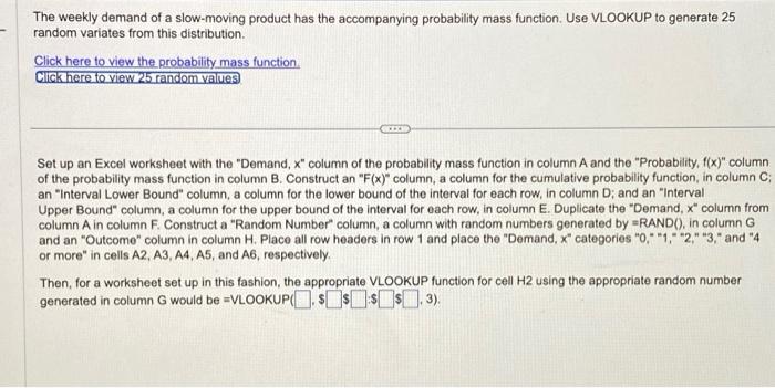
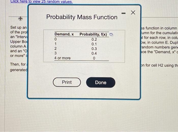
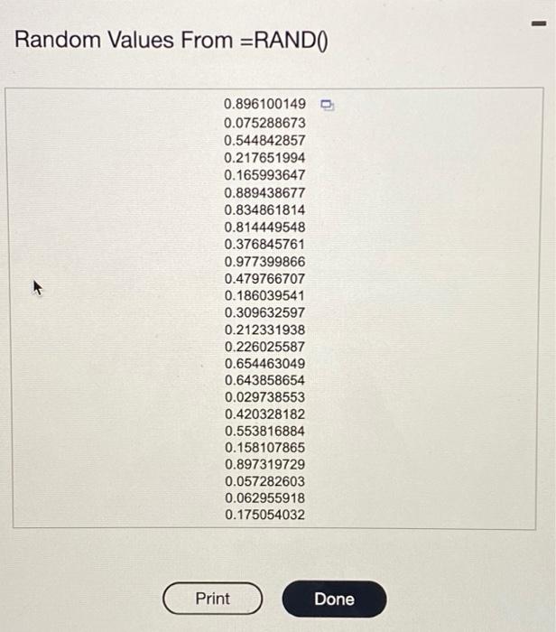
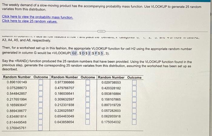
The weekly demand of a slow-moving product has the accompanying probability mass function. Use VLOOKUP to generate 25 random variates from this distribution. Click here to view the probability mass function Click here to view 25 random values Set up an Excel worksheet with the "Demand, x " column of the probability mass function in column A and the "Probability, f(x) " column an "Interval Lower Bound" column, a column for the lower bound of the interval for each row, in column D; and an "Interval Upper Bound" column, a column for the upper bound of the interval for each row, in column E. Duplicate the "Demand, x" column from column A in column F. Construct a "Random Number" column, a column with random numbers generated by =RAND(, in column G and an "Outcome" column in column H. Place all row headers in row 1 and place the "Demand, x " categories "0," "1," "2," "3," and "4 or more" in cells A2, A3, A4, A5, and A6, respectively. Then, for a worksheet set up in this fashion, the appropriate VLOOKUP function for cell H2 using the appropriate random number generated in column G would be =VLOOKUP $$$,3). $ Probability Mass Function ss function in column umn for the cumulati I for each row, in col ow, in column E. Dup andom numbers gen ree the "Demand, x" on for cell H2 using th Random Values From =RAND0 The weekly demand of a slow-moving product has the accompanying probability mass function. Use VLOOKUP to generate 25 random variates from this distribution. Click here to view the probability mass function. Click here to view 25 random values. A3,A4,A5, and A6, respectively. Then, for a worksheet set up in this fashion, the appropriate VLOOKUP function for cell H2 using the appropriate random number generated in column G would be =VLOOKUP (G2,$D$2:$F$5,3). Say the =RAND() function produced the 25 random numbers that have been provided. Using the VLOOKUP function found in the previous step, generate the corresponding 25 random variates from this distribution, assuming the worksheet has been set up as described. The weekly demand of a slow-moving product has the accompanying probability mass function. Use VLOOKUP to generate 25 random variates from this distribution. Click here to view the probability mass function Click here to view 25 random values Set up an Excel worksheet with the "Demand, x " column of the probability mass function in column A and the "Probability, f(x) " column an "Interval Lower Bound" column, a column for the lower bound of the interval for each row, in column D; and an "Interval Upper Bound" column, a column for the upper bound of the interval for each row, in column E. Duplicate the "Demand, x" column from column A in column F. Construct a "Random Number" column, a column with random numbers generated by =RAND(, in column G and an "Outcome" column in column H. Place all row headers in row 1 and place the "Demand, x " categories "0," "1," "2," "3," and "4 or more" in cells A2, A3, A4, A5, and A6, respectively. Then, for a worksheet set up in this fashion, the appropriate VLOOKUP function for cell H2 using the appropriate random number generated in column G would be =VLOOKUP $$$,3). $ Probability Mass Function ss function in column umn for the cumulati I for each row, in col ow, in column E. Dup andom numbers gen ree the "Demand, x" on for cell H2 using th Random Values From =RAND0 The weekly demand of a slow-moving product has the accompanying probability mass function. Use VLOOKUP to generate 25 random variates from this distribution. Click here to view the probability mass function. Click here to view 25 random values. A3,A4,A5, and A6, respectively. Then, for a worksheet set up in this fashion, the appropriate VLOOKUP function for cell H2 using the appropriate random number generated in column G would be =VLOOKUP (G2,$D$2:$F$5,3). Say the =RAND() function produced the 25 random numbers that have been provided. Using the VLOOKUP function found in the previous step, generate the corresponding 25 random variates from this distribution, assuming the worksheet has been set up as described