Please help!!! With explanation please.

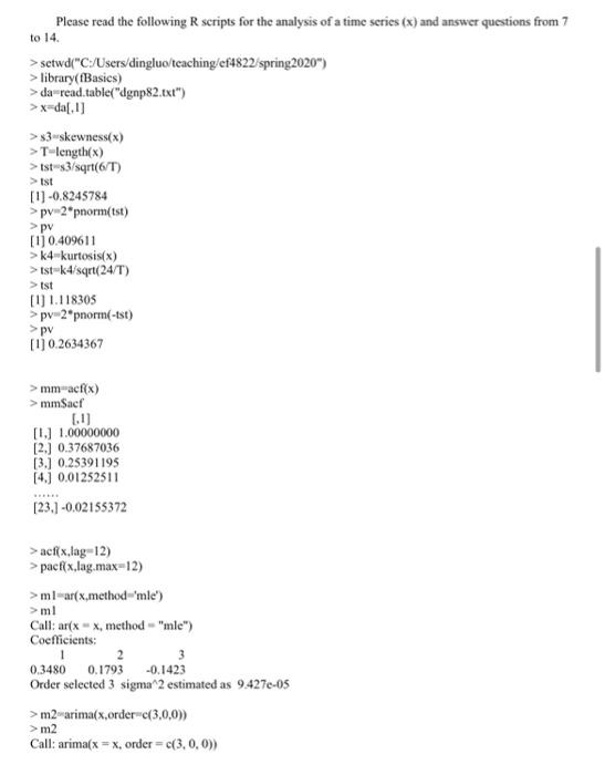
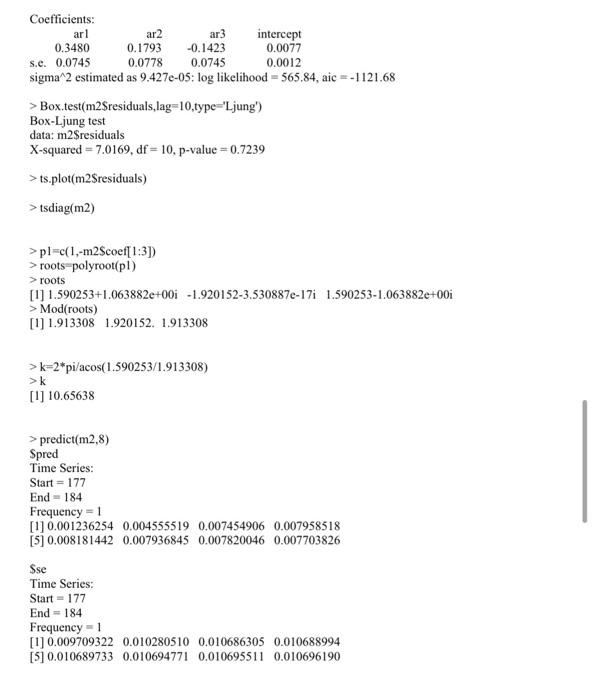
Please read the following scripts for the analysis of a time series (x) and answer questions from 7 to 14. >setwd("C:/Users/dingluo/teaching/ef4822 spring2020") > library(fBasics) >da read.table("dgnp82.txt") >xda[1] > 3 skewness(x) > T-length(x) >tst3/sqrt(6/T) >tst [1] -0.8245784 >pv 2*pnorm(st) >pv [10.409611 > K4-kurtosis(x) > tst-k4/sqrt(24/T) > Ist LU 1.118305 > pv2*pnorm(-tst) >pv [10.2634367 > mm-acf(x) > mmSacf 6.11 [1.] 1.00000000 [2.) 0.37687036 [3.] 0.25391195 [4.3 0.01252511 [23.7 -0.02155372 > acfix.lag-12) >pacf(x,lag.max-12) >mlar(x,methodmie) >ml Call: ar( xx, method "mle") Coefficients: 1 2 0.3480 0.1793 -0.1423 Order selected 3 sigma 2 estimated as 9.4270-05 > m2 arimax.order(3,0,0)) > m2 Call: arima(x = x, order=c(3, 0, 0)) Coefficients: arl ar2 ar3 intercept 0.3480 0.1793 -0.1423 0.0077 s.e. 0.0745 0.0778 0.0745 0.0012 sigma 2 estimated as 9.427e-05: log likelihood = 565.84, aic =-1121.68 > Box.test(m2$residuals,lag=10 type="Ljung') Box-Ljung test data: m2$residuals X-squared -7.0169, df = 10, p-value - 0.7239 > ts.plot(m2Sresiduals) > tsdiag(m2) >pl=c(1,-m2$coef[1:3]) > roots polyroot(pl) >roots [1] 1.590253+1.063882e+00i - 1.920152-3.5308870-176 1.590253-1.063882e-001 > Mod(roots) [1] 1.913308 1.920152. 1.913308 >k=2*pi/acos(1.590253/1.913308) > [1] 10.65638 > predict(m2,8) Spred Time Series: Start = 177 End - 184 Frequency - 1 [1] 0.001236254 0.004555519 0.007454906 0.007958518 [5] 0.008181442 0.007936845 0.007820046 0.007703826 Sse Time Series: Start = 177 End = 184 Frequency = 1 [1] 0.009709322 0.010280510 0.010686305 0.010688994 [5] 0.010689733 0.010694771 0.010695511 0.010696190 7. Is the distribution of the time series (x) skewed at 5% significance level? a yes b.no c. not sure 8. Does the distribution of the time series (x) have heavy tails at 5% significance level? a. yes b.no c. not sure 9. Which is the lag-2 autocorrelation of the time series (x)? a. 1.00000000 b. 0.37687036 c. 0.25391195 d. 0.01252511 10. Which is the specified and estimated model for the time series (x)? a. MA(3) b. AR(3) c. ARMA(1,2) d. ARMA(2,1) 11. Which is the mean of the time series (x)? a. 0.0077 b. 0.01180982 c. 0.02330508 d. 0.01252033 12. Which is the variance of the time series (x)? a. 0.00009427 b. 0.0001072596 c. 0.0001140595 d. 0.0001087317 13. Which is/are used to check whether the estimated model is adequate? a. tsdiag(m2) b. Box.test(m2$residuais, lag 10,type="Ljung) c. predict(m2,8) d. both a and b Please read the following scripts for the analysis of a time series (x) and answer questions from 7 to 14. >setwd("C:/Users/dingluo/teaching/ef4822 spring2020") > library(fBasics) >da read.table("dgnp82.txt") >xda[1] > 3 skewness(x) > T-length(x) >tst3/sqrt(6/T) >tst [1] -0.8245784 >pv 2*pnorm(st) >pv [10.409611 > K4-kurtosis(x) > tst-k4/sqrt(24/T) > Ist LU 1.118305 > pv2*pnorm(-tst) >pv [10.2634367 > mm-acf(x) > mmSacf 6.11 [1.] 1.00000000 [2.) 0.37687036 [3.] 0.25391195 [4.3 0.01252511 [23.7 -0.02155372 > acfix.lag-12) >pacf(x,lag.max-12) >mlar(x,methodmie) >ml Call: ar( xx, method "mle") Coefficients: 1 2 0.3480 0.1793 -0.1423 Order selected 3 sigma 2 estimated as 9.4270-05 > m2 arimax.order(3,0,0)) > m2 Call: arima(x = x, order=c(3, 0, 0)) Coefficients: arl ar2 ar3 intercept 0.3480 0.1793 -0.1423 0.0077 s.e. 0.0745 0.0778 0.0745 0.0012 sigma 2 estimated as 9.427e-05: log likelihood = 565.84, aic =-1121.68 > Box.test(m2$residuals,lag=10 type="Ljung') Box-Ljung test data: m2$residuals X-squared -7.0169, df = 10, p-value - 0.7239 > ts.plot(m2Sresiduals) > tsdiag(m2) >pl=c(1,-m2$coef[1:3]) > roots polyroot(pl) >roots [1] 1.590253+1.063882e+00i - 1.920152-3.5308870-176 1.590253-1.063882e-001 > Mod(roots) [1] 1.913308 1.920152. 1.913308 >k=2*pi/acos(1.590253/1.913308) > [1] 10.65638 > predict(m2,8) Spred Time Series: Start = 177 End - 184 Frequency - 1 [1] 0.001236254 0.004555519 0.007454906 0.007958518 [5] 0.008181442 0.007936845 0.007820046 0.007703826 Sse Time Series: Start = 177 End = 184 Frequency = 1 [1] 0.009709322 0.010280510 0.010686305 0.010688994 [5] 0.010689733 0.010694771 0.010695511 0.010696190 7. Is the distribution of the time series (x) skewed at 5% significance level? a yes b.no c. not sure 8. Does the distribution of the time series (x) have heavy tails at 5% significance level? a. yes b.no c. not sure 9. Which is the lag-2 autocorrelation of the time series (x)? a. 1.00000000 b. 0.37687036 c. 0.25391195 d. 0.01252511 10. Which is the specified and estimated model for the time series (x)? a. MA(3) b. AR(3) c. ARMA(1,2) d. ARMA(2,1) 11. Which is the mean of the time series (x)? a. 0.0077 b. 0.01180982 c. 0.02330508 d. 0.01252033 12. Which is the variance of the time series (x)? a. 0.00009427 b. 0.0001072596 c. 0.0001140595 d. 0.0001087317 13. Which is/are used to check whether the estimated model is adequate? a. tsdiag(m2) b. Box.test(m2$residuais, lag 10,type="Ljung) c. predict(m2,8) d. both a and b