Please help with Problem 2 only. Problem 1 just for reference.

Reference Problem 1:

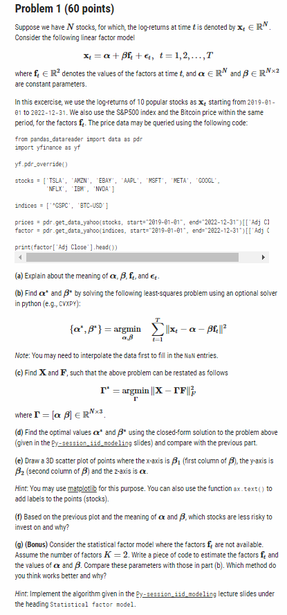
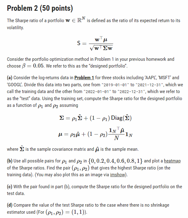
The Sharpe ratio of a portfolio wRN is defined as the ratio of its expected return to its volatility. S=www Consider the portfolio optimization method in Problem 1 in your previous homework and choose =0.05. We refer to this as the "designed portfolio". (a) Consider the log-returns data in Problem 1 for three stocks including 'AAPL', 'MSFT' and 'G00GL'. Divide this data into two parts, one from "2019-01-01" to "2021-12-31", which we call the training data and the other from "2022-01-01" to "2022-12-31", which we refer to as the "test" data. Using the training set, compute the Sharpe ratio for the designed portfolio as a function of 1 and 2 assuming =1^+(11)Diag(^)=2^+(12)N1N^1N where ^ is the sample covariance matrix and ^ is the sample mean. (b) Use all possible pairs for 1 and 2 in {0,0.2,0.4,0.6,0.8,1} and plot a heatmap of the Sharpe ratios. Find the pair (1,2) that gives the highest Sharpe ratio (on the training data). (You may also plot this as an image via imshow). (c) With the pair found in part (b), compute the Sharpe ratio for the designed portfolio on the test data. (d) Compare the value of the test Sharpe ratio to the case where there is no shrinkage estimator used (For (1,2)=(1,1)) Suppose we have N stocks, for which, the log-returns at time t is denoted by xtRN. Consider the following linear factor model xt=+ft+t,t=1,2,,T where ftR2 denotes the values of the factors at time t, and RN and RN2 are constant parameters. In this excercise, we use the log-returns of 10 popular stocks as xt starting from 2019-01 01 to 20221231. We also use the S\&P500 index and the Bitcoin price within the same period, for the factors ft. The price data may be queried using the following code: from pandas_datareader import data as pdr import yfinance as yf yf.pdr_override() stocks = I'TSLA', 'AMZN', 'EBAY', 'AAPL', 'MSFT', 'NETA', 'GOOGL', 'NFLX', 'IBY', 'NVDA'] indices =[ ' "GSPC', 'BTC-USD' ] prices = pdr -get_data_yahoo(stocks, start="2019-01-01", end="2022-12-31") [['Adj CI factor = pdr.get_data_yahoo(indices, start="2019-61-01", end="2922-12-31") [['Adj C print(factor['Adj Close'].head( ) ) (a) Explain about the meaning of ,,ft, and t. (b) Find and 4 by solving the following least-squares problem using an optional solver in python (e.9., cvxpy): {,}=,argmint=1Txtft2 Note: You may need to interpolate the data first to fill in the NaN entries. (c) Find X and F, such that the above problem can be restated as follows =rargminXFF2 where =[]RN3. (d) Find the optimal values 4 and +using the closed-form solution to the problem above (given in the Py_session_iid_node ling slides) and compare with the previous part. (e) Draw a 3D scatter plot of points where the x-axis is 1 (first column of ), the y-axis is 2 (second column of ) and the z-axis is . Hint. You may use matplotilib for this purpose. You can also use the function ax text() to add labels to the points (stocks). (f) Based on the previous plot and the meaning of and , which stocks are less risky to invest on and why? (g) (Bonus) Consider the statistical factor model where the factors ft are not available. Assume the number of factors K=2. Write a piece of code to estimate the factors ft and the values of and . Compare these parameters with those in part (b). Which method do you think works better and why? Hint. Implement the algorithm given in the Py_session_iid_modeling lecture slides under the heading Statistical factor model