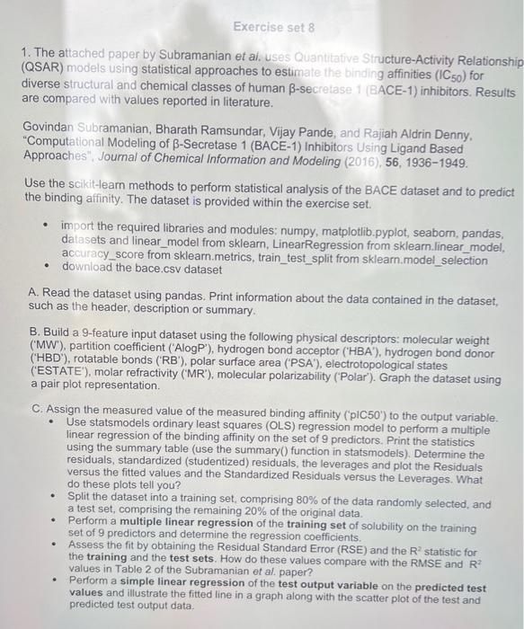
please include code and dataset name is "bace.csv", please include in code!

Exercise set 8 1. The attached paper by Subramanian et ai. uses Quantitative Structure-Activity Relationsh (QSAR) models using statistical approaches to estimate the binding affinities (IC50) for diverse siructural and chemical classes of human -secretase 1 (BACE-1) inhibitors. Results are compared with values reported in literature. Govindan Subramanian, Bharath Ramsundar, Vijay Pande, and Rajiah Aldrin Denny, "Computational Modeling of -Secretase 1 (BACE-1) Inhibitors Using Ligand Based Approaches", Joumal of Chemical Information and Modeling (2016),56, 1936-1949. Use the scikit-learn methods to perform statistical analysis of the BACE dataset and to predict the binding affinity. The dataset is provided within the exercise set. - import the required libraries and modules: numpy, matplotlib.pyplot, seaborn, pandas, datasets and linear_model from sklearn, LinearRegression from sklearn.linear_model, accuracy_score from sklearn.metrics, train_test_split from sklearn.model_selection - downioad the bace.csv dataset A. Read the dataset using pandas. Print information about the data contained in the dataset, such as the header, description or summary. B. Build a 9-feature input dataset using the following physical descriptors: molecular weight ('MW'), partition coefficient ('AlogP'), hydrogen bond acceptor ('HBA'), hydrogen bond donor ('HBD'), rotatable bonds ('RB'), polar surface area ('PSA'), electrotopological states ('ESTATE'), molar refractivity ('MR'), molecular polarizability ('Polar'). Graph the dataset using a pair plot representation. C. Assign the measured value of the measured binding affinity ('pIC50') to the output variable. - Use statsmodels ordinary least squares (OLS) regression model to perform a multiple linear regression of the binding affinity on the set of 9 predictors. Print the statistics using the summary table (use the summary() function in statsmodels). Determine the residuals, standardized (studentized) residuals, the leverages and plot the Residuals versus the fitted values and the Standardized Residuals versus the Leverages. What do these plots tell you? - Split the dataset into a training set, comprising 80% of the data randomly selected, and a test set, comprising the remaining 20% of the original data. - Perform a multiple linear regression of the training set of solubility on the training set of 9 predictors and determine the regression coefficients. - Assess the fit by obtaining the Residual Standard Error (RSE) and the R2 statistic for the training and the test sets. How do these values compare with the RMSE and R2 values in Table 2 of the Subramanian et al. paper? - Perform a simple linear regression of the test output variable on the predicted test values and illustrate the fitted line in a graph along with the scatter plot of the test and predicted test output data. D. Generate an 3 single-feature datasets by selecting only the column ' MW ', or 'HBD', or 'Estate' from the above set in part B. - Perform a single linear regression on each of the single-feature datasets using the approach in part C. - How do the results for each simple linear regression compare with the multiple linear regression from part C