Please Label two points on the graph that a whole integers in both the X and Y axis.

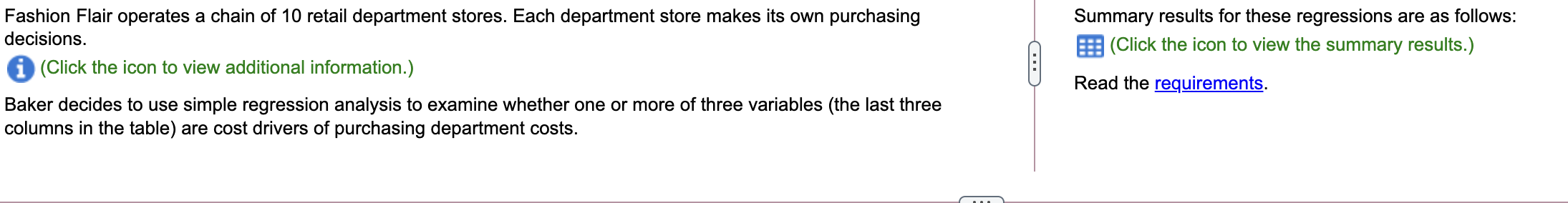
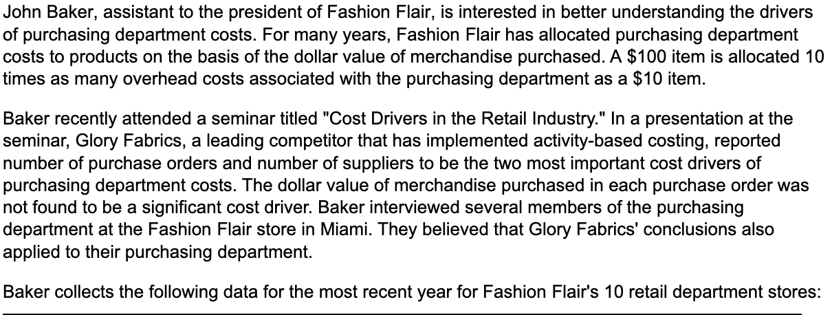
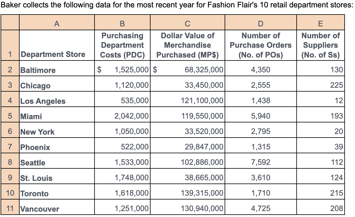
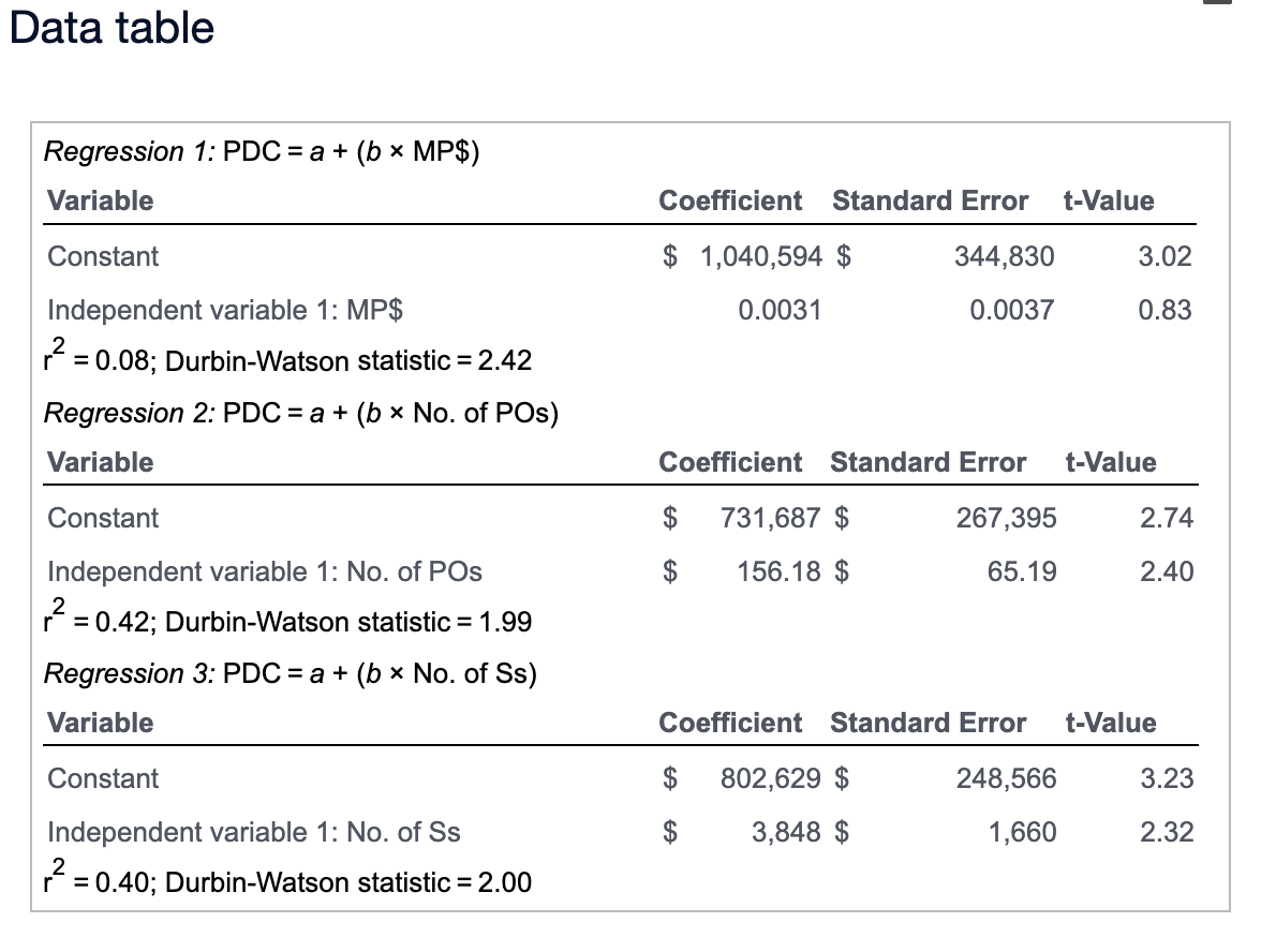
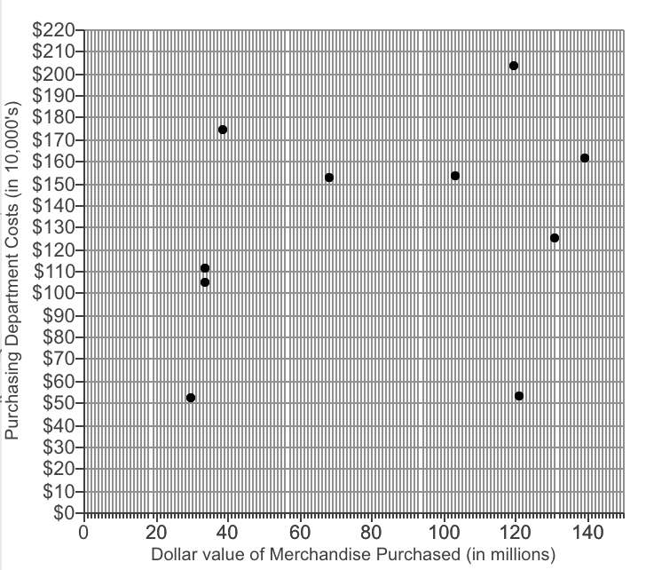
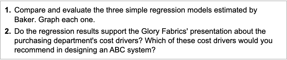
Fashion Flair operates a chain of 10 retail department stores. Each department store makes its own purchasing decisions. (Click the icon to view additional information.) Summary results for these regressions are as follows: (Click the icon to view the summary results.) E Read the requirements. Baker decides to use simple regression analysis to examine whether one or more of three variables (the last three columns in the table) are cost drivers of purchasing department costs. John Baker, assistant to the president of Fashion Flair, is interested in better understanding the drivers of purchasing department costs. For many years, Fashion Flair has allocated purchasing department costs to products on the basis of the dollar value of merchandise purchased. A $100 item is allocated 10 times as many overhead costs associated with the purchasing department as a $10 item. Baker recently attended a seminar titled "Cost Drivers in the Retail Industry." In a presentation at the seminar, Glory Fabrics, a leading competitor that has implemented activity-based costing, reported number of purchase orders and number of suppliers to be the two most important cost drivers of purchasing department costs. The dollar value of merchandise purchased in each purchase order was not found to be a significant cost driver. Baker interviewed several members of the purchasing department at the Fashion Flair store in Miami. They believed that Glory Fabrics' conclusions also applied to their purchasing department. Baker collects the following data for the most recent year for Fashion Flair's 10 retail department stores: Baker collects the following data for the most recent year for Fashion Flair's 10 retail department stores: A B D E Number of Purchase Orders (No. of POs) Number of Suppliers (No. of Ss) 1 Department Store Purchasing Dollar Value of Department Merchandise Costs (PDC) Purchased (MP) $ 1,525,000 $ 68,325,000 1,120,000 33,450,000 2 Baltimore 4,350 130 3 Chicago 2,555 225 4 Los Angeles 535,000 121,100,000 1,438 12 5 Miami 2,042,000 119,550,000 5,940 193 6 New York 1,050,000 33,520,000 2,795 20 7 Phoenix 522,000 29,847,000 1,315 39 8 Seattle 1,533,000 102,886,000 7,592 112 9 St. Louis 1,748,000 38,665,000 3,610 124 10 Toronto 1,618,000 139,315,000 1,710 215 11 Vancouver 1,251,000 130,940,000 4,725 208 Data table Regression 1: PDC = a + (6 ~ MP$) Variable Coefficient Standard Error t-Value Constant $ 1,040,594 $ 344,830 3.02 0.0031 0.0037 0.83 Independent variable 1: MP$ p = = 0.08; Durbin-Watson statistic = 2.42 Regression 2: PDC = a + (6 * No. of POs) Variable Coefficient Standard Error t-Value Constant $ 731,687 $ 267,395 2.74 $ 156.18 $ 65.19 2.40 r = Independent variable 1: No. of POS 2 = 0.42; Durbin-Watson statistic = 1.99 Regression 3: PDC = a + (6 * No. of Ss) Variable Coefficient Standard Error t-Value Constant $ 802,629 $ 248,566 3.23 3,848 $ 1,660 2.32 Independent variable 1: No. of Ss 2 = 0.40; Durbin-Watson statistic = 2.00 Purchasing Department Costs (in 10,000's) $220- $210- $200- $190- $180- $170- $160- 5 $150- $140- $130- $120- $110- $100- $90- $80- $70- $60- $50- $40- $30- $20- $10- $0- 0 140 20 40 60 80 100 120 Dollar value of Merchandise Purchased (in millions) 1. Compare and evaluate the three simple regression models estimated by Baker. Graph each one. 2. Do the regression results support the Glory Fabrics' presentation about the purchasing department's cost drivers? Which of these cost drivers would you recommend in designing an ABC system? Fashion Flair operates a chain of 10 retail department stores. Each department store makes its own purchasing decisions. (Click the icon to view additional information.) Summary results for these regressions are as follows: (Click the icon to view the summary results.) E Read the requirements. Baker decides to use simple regression analysis to examine whether one or more of three variables (the last three columns in the table) are cost drivers of purchasing department costs. John Baker, assistant to the president of Fashion Flair, is interested in better understanding the drivers of purchasing department costs. For many years, Fashion Flair has allocated purchasing department costs to products on the basis of the dollar value of merchandise purchased. A $100 item is allocated 10 times as many overhead costs associated with the purchasing department as a $10 item. Baker recently attended a seminar titled "Cost Drivers in the Retail Industry." In a presentation at the seminar, Glory Fabrics, a leading competitor that has implemented activity-based costing, reported number of purchase orders and number of suppliers to be the two most important cost drivers of purchasing department costs. The dollar value of merchandise purchased in each purchase order was not found to be a significant cost driver. Baker interviewed several members of the purchasing department at the Fashion Flair store in Miami. They believed that Glory Fabrics' conclusions also applied to their purchasing department. Baker collects the following data for the most recent year for Fashion Flair's 10 retail department stores: Baker collects the following data for the most recent year for Fashion Flair's 10 retail department stores: A B D E Number of Purchase Orders (No. of POs) Number of Suppliers (No. of Ss) 1 Department Store Purchasing Dollar Value of Department Merchandise Costs (PDC) Purchased (MP) $ 1,525,000 $ 68,325,000 1,120,000 33,450,000 2 Baltimore 4,350 130 3 Chicago 2,555 225 4 Los Angeles 535,000 121,100,000 1,438 12 5 Miami 2,042,000 119,550,000 5,940 193 6 New York 1,050,000 33,520,000 2,795 20 7 Phoenix 522,000 29,847,000 1,315 39 8 Seattle 1,533,000 102,886,000 7,592 112 9 St. Louis 1,748,000 38,665,000 3,610 124 10 Toronto 1,618,000 139,315,000 1,710 215 11 Vancouver 1,251,000 130,940,000 4,725 208 Data table Regression 1: PDC = a + (6 ~ MP$) Variable Coefficient Standard Error t-Value Constant $ 1,040,594 $ 344,830 3.02 0.0031 0.0037 0.83 Independent variable 1: MP$ p = = 0.08; Durbin-Watson statistic = 2.42 Regression 2: PDC = a + (6 * No. of POs) Variable Coefficient Standard Error t-Value Constant $ 731,687 $ 267,395 2.74 $ 156.18 $ 65.19 2.40 r = Independent variable 1: No. of POS 2 = 0.42; Durbin-Watson statistic = 1.99 Regression 3: PDC = a + (6 * No. of Ss) Variable Coefficient Standard Error t-Value Constant $ 802,629 $ 248,566 3.23 3,848 $ 1,660 2.32 Independent variable 1: No. of Ss 2 = 0.40; Durbin-Watson statistic = 2.00 Purchasing Department Costs (in 10,000's) $220- $210- $200- $190- $180- $170- $160- 5 $150- $140- $130- $120- $110- $100- $90- $80- $70- $60- $50- $40- $30- $20- $10- $0- 0 140 20 40 60 80 100 120 Dollar value of Merchandise Purchased (in millions) 1. Compare and evaluate the three simple regression models estimated by Baker. Graph each one. 2. Do the regression results support the Glory Fabrics' presentation about the purchasing department's cost drivers? Which of these cost drivers would you recommend in designing an ABC system