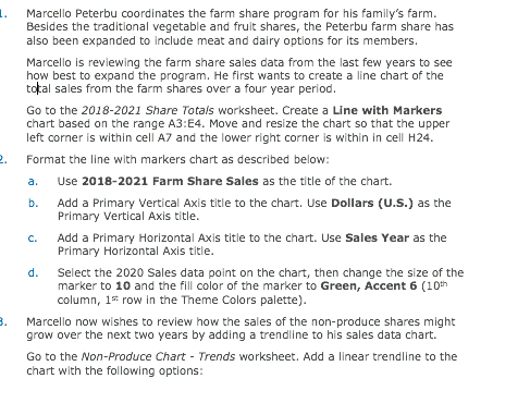
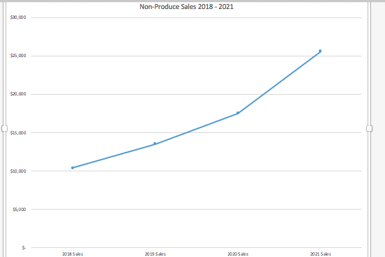
Please list what I should do for each step.

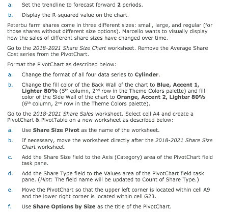
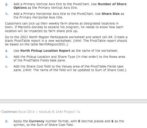
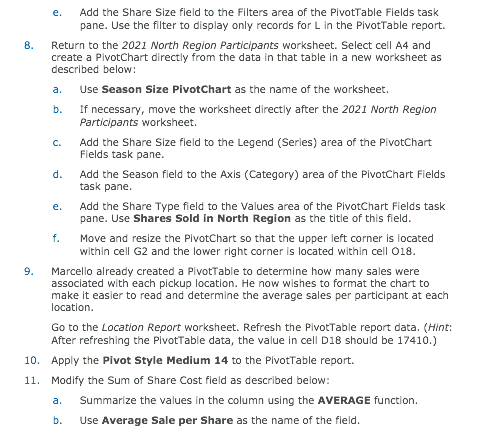
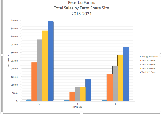
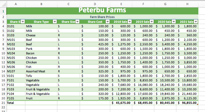
Set the trendline to forecast forward 2 periods. Display the R-squared value on the chart. a. b. Peterbu farm shares come in three different sizes: small, large, and regular (for those shares without different size options). Marcello wants to visually display how the sales of different share sizes have changed over time Go to the 2018-2021 Share Size Chart worksheet. Remove the Average Share Cost series from the PlvotChart. Format the PlvotChart as described below: a. Change the format of all four data serles to Cylinder b. Change the fill color of the Back Wall of the chart to Blue, Accent 1, Lighter 80% (5th column, 2nd row in the Theme Colors palette) and fill color of the side wall of the chart to Orange, Accent 2, Lighter 80% (6th column, 2nd row in the Theme Colors palette) Go to the 2018-2021 Share Sales worksheet. Select cell A4 and create a PlvotChart & PivotTable on a new worksheet as described below: a. Use Share Size Pivot as the name of the worksheet b. If necessary, move the worksheet directly after the 2018-2021 Share Size Chart worksheet. Add the Share Size field to the Axis (Category) area of the PivotChart field task pane c. d Add the Share Type field to the Values area of the PivotChart field task pane. (Hint: The field name wl be updated to Count of Share Type.) Move the PivotChart so that the upper left corner is located within cell A9 and the lower right corner is located within cell G23 Use Share Options by Size as the title of the PivotChart. e. f. g Add a Primary Vertical Axis title to the PivotChart. Use Number of Share Options as the Primary Vertical Axis title h. Add a Primary Horizontal Axis title to the PivotChart. Use Share Size as the Primary Horizontal Axis title Customers can pick up their weekly farm shares at designated locations in town. if Marcello decides to expand his program, he needs to know how each location will be impacted by farm share pick up Go to the 2021 North Region Particlpants worksheet and select cell A4. Create a blank PivotTable report in a new worksheet. (Hint: The PivotTable report should be based on the table NorthRegion2021.) a. Use North Pickup Location Report as the name of the worksheet. b. Add the Pickup Location and Share Type in that order) to the Rows area of the PivotTable Fields task pane. Add the Share Cost fleld to the Values area of the PivotTable Fields task pane. (Hint: The name of the field will be updated to Sum of Share Cost.) c. Cashman Excel 2016 | Module 8: SAM Project la d Apply the Currency number format, with 0 decimal places and $ as the symbol, to the Sum of Share Cost field Add the Share Size field to the Filters area of the PlvotTable Flelds task pane. Use the filter to display only records for L in the PivotTable report. e. 8 Return to the 2021 North Region Partlclpants worksheet. Select cell A4 and create a PivotChart directly from the data in that table in a new worksheet as described below: a Use Season Size PivotChart as the name of the worksheet. b. If necessary, move the worksheet directly after the 2021 North Region Participants worksheet. Add the Share Size field to the Legend (Serles) area of the PivotChart Fields task pane Add the Season field to the Axis (Category) area of the PivotChart Fields task pane Add the Share Type field to the Values area of the PivotChart Fields task pane. Use Shares Sold in North Region as the title of this field Move and resize the PlvotChart so that the upper left corner is located within cell G2 and the lower right corner is located within cell O18 c. d. e. f. 9 Marcello already created a PlvotTable to determine how many sales were associated with each pickup location. He now wishes to format the chart to make it easler to read and determine the average sales per participant at each location. Go to the Location Report worksheet. Refresh the PivotTable report data. (Hint: After refreshing the PivotTable data, the value in cell D18 should be 17410.) 10. Apply the Pivot Style Medium 14 to the PivotTable report. 11. Modify the Sum of Share Cost field as described below Summarize the values in the column using the AVERAGE function. Use Average Sale per Share as the name of the field a. b. 12. Modify the number format of the Total Share Sales field, so that the values display in the Accounting number format, with 0 decimal places and as the symbol 13. 14. Change the Report Layout so that the report is viewed in Outline Form. Switch to the Sales Total Report worksheet. Each customer has purchased the same farm share package each year they have participated in the program. Add a new calculated field to the end of the PivotTable report to calculate the cumulative share sales for each customer as described below: Create a formula without using a function that multiplies the Share Cost by the Years Participating. (Hint: The calculated field will automatically be added to your PivotTable.) a. b. Apply the Accounting number format, with 0 decimal places and the $ symbol, to the newly created column. Shelly Cashman Excel 2016 1 Module 8: SAM Project 1a c. Use Cumulative Share Sales as the custom name of the field. 15. Go to the Share Type Report worksheet. Format the Season Slicer as described below: a. Format the Slicer using the Slicer Style Light 6 15. Go to the Share Type Report worksheet. Format the Season Slicer as described below a. Format the Slicer using the Slicer Style Light 6 b. Use the Slicer to filter the PivotTable report to display only data for the Summer-Fall field 16. Add another Slicer to the Model PivotTable report based on the Share Type field, then complete the following actions: a. Resize and reposition the Share Type Slicer, so that the upper left corner is located within cell D10 and the lower right corner is located within cell G26 b. Format the Slicer using the Slicer Style Light 6 c. Use the Slicer to filter the PivotTable report to display only data for Fruit, Fruit & Vegetable, and Vegetable fields. (Hint: The PlvotTable should already be filtered using the Season Slicer.) Non-Produce Sales 2018- 2021 30,000 $25,000 sis,000 10,000 $5,000 2038 5aes 20205 aes 2021 Sales Peterbu Farms Total Sales by Farm Share Size 2018-2021 $50,000 $45,000 A0,000 35,000 $30,000 Share Cost Total 2018 Sales Total 2019 Sales Total 2020 Sales 525,000 20,000 Total 2021 Sales $15,000 $10,000 55,000 SHARE SRE Peterbu Farms Farm Share Prices Share ID Share Type Share Size Share Cost 2018 Sale 2019 Sale 2020 Sale 2021 Sale Milk 100.00 600.00 $1,000.00 1,300.00 1,800.00 150.00 300.00 600.00 450.00 450.00 120.00 S 120.00 240.00 240.00 $ 360.00 300.00 300.00600.00 1,200.00$ 2,100.00 425.00 1,275.00 2,550.00 $ 3,400.00 4,250.00 300.00 600.00$ 1,500.001,800.00$ 1,800.00 250.00 1,250.00 $ 1,250.00 1,750.00 $ 3,500.00 250.00 1,000.00 1,000.00 1,250.003,000.00 350.00 1,750.00 1,400.00 1,750.00 3,850.00 200.00 400.00 600.00 1,000.00 1,000.00 325.00 975.00 $ 975.00 650.00 650.00 150.00 1,800.00 1,800.00 2,700.00 2,850.00 150.00 S 5,700.00 8,850.00 10,500.00 13,800.00 240.00 7,680.00 16,080.00 18,240.00 $ 19,680.00 200.00 $ 7,200.00 8,600.00 $ 11,400.00 10,200.00 320.00 12,800.0017,600.00 $19,840.00 21,440.00 175.00 $ 1,925.00 3,850.00 $ 2,975.00 6,125.00 45,675.00 68,495.00 80,445.00 96,855.00 4 D101 5 D102 6 D103 Beef Pork 9 M103 1104 11 M105 Chicken Chicken Fish Assorted Meat 13 M106 14 M107 16 P101 17 P102 18 P103 19 P104 20 P105 21 Total Vegetable Vegetable Fruit & Vegetable S Fruit & Vegetable Fruit Set the trendline to forecast forward 2 periods. Display the R-squared value on the chart. a. b. Peterbu farm shares come in three different sizes: small, large, and regular (for those shares without different size options). Marcello wants to visually display how the sales of different share sizes have changed over time Go to the 2018-2021 Share Size Chart worksheet. Remove the Average Share Cost series from the PlvotChart. Format the PlvotChart as described below: a. Change the format of all four data serles to Cylinder b. Change the fill color of the Back Wall of the chart to Blue, Accent 1, Lighter 80% (5th column, 2nd row in the Theme Colors palette) and fill color of the side wall of the chart to Orange, Accent 2, Lighter 80% (6th column, 2nd row in the Theme Colors palette) Go to the 2018-2021 Share Sales worksheet. Select cell A4 and create a PlvotChart & PivotTable on a new worksheet as described below: a. Use Share Size Pivot as the name of the worksheet b. If necessary, move the worksheet directly after the 2018-2021 Share Size Chart worksheet. Add the Share Size field to the Axis (Category) area of the PivotChart field task pane c. d Add the Share Type field to the Values area of the PivotChart field task pane. (Hint: The field name wl be updated to Count of Share Type.) Move the PivotChart so that the upper left corner is located within cell A9 and the lower right corner is located within cell G23 Use Share Options by Size as the title of the PivotChart. e. f. g Add a Primary Vertical Axis title to the PivotChart. Use Number of Share Options as the Primary Vertical Axis title h. Add a Primary Horizontal Axis title to the PivotChart. Use Share Size as the Primary Horizontal Axis title Customers can pick up their weekly farm shares at designated locations in town. if Marcello decides to expand his program, he needs to know how each location will be impacted by farm share pick up Go to the 2021 North Region Particlpants worksheet and select cell A4. Create a blank PivotTable report in a new worksheet. (Hint: The PivotTable report should be based on the table NorthRegion2021.) a. Use North Pickup Location Report as the name of the worksheet. b. Add the Pickup Location and Share Type in that order) to the Rows area of the PivotTable Fields task pane. Add the Share Cost fleld to the Values area of the PivotTable Fields task pane. (Hint: The name of the field will be updated to Sum of Share Cost.) c. Cashman Excel 2016 | Module 8: SAM Project la d Apply the Currency number format, with 0 decimal places and $ as the symbol, to the Sum of Share Cost field Add the Share Size field to the Filters area of the PlvotTable Flelds task pane. Use the filter to display only records for L in the PivotTable report. e. 8 Return to the 2021 North Region Partlclpants worksheet. Select cell A4 and create a PivotChart directly from the data in that table in a new worksheet as described below: a Use Season Size PivotChart as the name of the worksheet. b. If necessary, move the worksheet directly after the 2021 North Region Participants worksheet. Add the Share Size field to the Legend (Serles) area of the PivotChart Fields task pane Add the Season field to the Axis (Category) area of the PivotChart Fields task pane Add the Share Type field to the Values area of the PivotChart Fields task pane. Use Shares Sold in North Region as the title of this field Move and resize the PlvotChart so that the upper left corner is located within cell G2 and the lower right corner is located within cell O18 c. d. e. f. 9 Marcello already created a PlvotTable to determine how many sales were associated with each pickup location. He now wishes to format the chart to make it easler to read and determine the average sales per participant at each location. Go to the Location Report worksheet. Refresh the PivotTable report data. (Hint: After refreshing the PivotTable data, the value in cell D18 should be 17410.) 10. Apply the Pivot Style Medium 14 to the PivotTable report. 11. Modify the Sum of Share Cost field as described below Summarize the values in the column using the AVERAGE function. Use Average Sale per Share as the name of the field a. b. 12. Modify the number format of the Total Share Sales field, so that the values display in the Accounting number format, with 0 decimal places and as the symbol 13. 14. Change the Report Layout so that the report is viewed in Outline Form. Switch to the Sales Total Report worksheet. Each customer has purchased the same farm share package each year they have participated in the program. Add a new calculated field to the end of the PivotTable report to calculate the cumulative share sales for each customer as described below: Create a formula without using a function that multiplies the Share Cost by the Years Participating. (Hint: The calculated field will automatically be added to your PivotTable.) a. b. Apply the Accounting number format, with 0 decimal places and the $ symbol, to the newly created column. Shelly Cashman Excel 2016 1 Module 8: SAM Project 1a c. Use Cumulative Share Sales as the custom name of the field. 15. Go to the Share Type Report worksheet. Format the Season Slicer as described below: a. Format the Slicer using the Slicer Style Light 6 15. Go to the Share Type Report worksheet. Format the Season Slicer as described below a. Format the Slicer using the Slicer Style Light 6 b. Use the Slicer to filter the PivotTable report to display only data for the Summer-Fall field 16. Add another Slicer to the Model PivotTable report based on the Share Type field, then complete the following actions: a. Resize and reposition the Share Type Slicer, so that the upper left corner is located within cell D10 and the lower right corner is located within cell G26 b. Format the Slicer using the Slicer Style Light 6 c. Use the Slicer to filter the PivotTable report to display only data for Fruit, Fruit & Vegetable, and Vegetable fields. (Hint: The PlvotTable should already be filtered using the Season Slicer.) Non-Produce Sales 2018- 2021 30,000 $25,000 sis,000 10,000 $5,000 2038 5aes 20205 aes 2021 Sales Peterbu Farms Total Sales by Farm Share Size 2018-2021 $50,000 $45,000 A0,000 35,000 $30,000 Share Cost Total 2018 Sales Total 2019 Sales Total 2020 Sales 525,000 20,000 Total 2021 Sales $15,000 $10,000 55,000 SHARE SRE Peterbu Farms Farm Share Prices Share ID Share Type Share Size Share Cost 2018 Sale 2019 Sale 2020 Sale 2021 Sale Milk 100.00 600.00 $1,000.00 1,300.00 1,800.00 150.00 300.00 600.00 450.00 450.00 120.00 S 120.00 240.00 240.00 $ 360.00 300.00 300.00600.00 1,200.00$ 2,100.00 425.00 1,275.00 2,550.00 $ 3,400.00 4,250.00 300.00 600.00$ 1,500.001,800.00$ 1,800.00 250.00 1,250.00 $ 1,250.00 1,750.00 $ 3,500.00 250.00 1,000.00 1,000.00 1,250.003,000.00 350.00 1,750.00 1,400.00 1,750.00 3,850.00 200.00 400.00 600.00 1,000.00 1,000.00 325.00 975.00 $ 975.00 650.00 650.00 150.00 1,800.00 1,800.00 2,700.00 2,850.00 150.00 S 5,700.00 8,850.00 10,500.00 13,800.00 240.00 7,680.00 16,080.00 18,240.00 $ 19,680.00 200.00 $ 7,200.00 8,600.00 $ 11,400.00 10,200.00 320.00 12,800.0017,600.00 $19,840.00 21,440.00 175.00 $ 1,925.00 3,850.00 $ 2,975.00 6,125.00 45,675.00 68,495.00 80,445.00 96,855.00 4 D101 5 D102 6 D103 Beef Pork 9 M103 1104 11 M105 Chicken Chicken Fish Assorted Meat 13 M106 14 M107 16 P101 17 P102 18 P103 19 P104 20 P105 21 Total Vegetable Vegetable Fruit & Vegetable S Fruit & Vegetable Fruit