Please provide step by step process

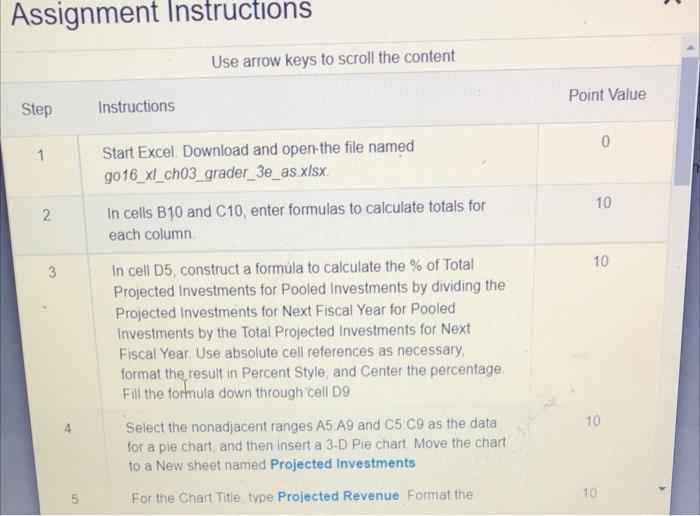
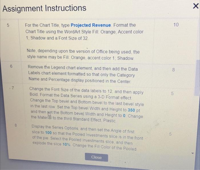
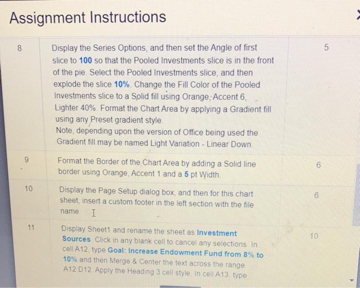
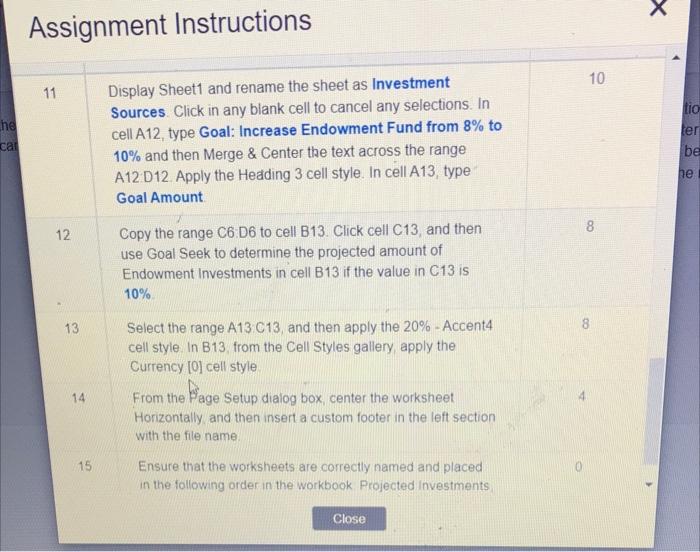
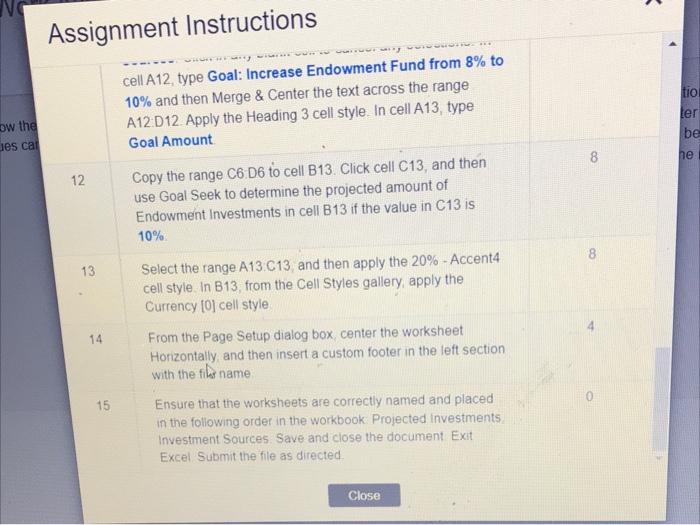
Assignment Instructions Use arrow keys to scroll the content Point Value Step Instructions 0 1 Start Excel. Download and open the file named go16_xl_ch03_grader_3e_as.x/sx. In cells B10 and C10, enter formulas to calculate totals for each column 10 2 10 3 In cell D5, construct a formula to calculate the % of Total Projected Investments for Pooled Investments by dividing the Projected Investments for Next Fiscal Year for Pooled Investments by the Total Projected Investments for Next Fiscal Year Use absolute cell references as necessary format the result in Percent Style and Center the percentage Fill the formula down through cell D9 10 4 Select the nonadjacent ranges A5 A9 and C5 C9 as the data for a pie chart, and then insert a 3-D Pie chart. Move the chart to a New sheet named Projected Investments 5 For the Chart Title type Projected Revenue Format the 10 Assignment Instructions 5 10 For the Chart Title type Projected Revenue Format the Chart Title using the WordArt Style Fill: Orange, Accent color 1 Shadow and a Font Size of 32 Note, depending upon the version of Office being used the style name may be Fill Orange, accent color 1: Shadow 6 8 Remove the Legend chart element, and then add the Data Labels chart element formatted so that only the Category Name and Percentage display positioned in the Center ..7 5 Change the Font Size of the data labels to 12 and then apply Bold. Format the Data Senes using a 3-D Format effect Change the Top bevel and Bottom bevel to the last bevel style in the last row Set the Top bevel Width and Height to 350 pt and then get the Bottom bevej Width and Height to 0 Change the Material to the third Standard Effect Plastic Display the Series Options and then set the Angle of first slice to 100 so that the Pooled investments slice is in the front of the pie. Select the Pooled Investments slice, and then explode the slice 10% Change the Fill Color of the Pooled 5. Close Assignment Instructions 8 5 Display the Series Options, and then set the Angle of first slice to 100 so that the Pooled Investments slice is in the front of the pie Select the Pooled Investments slice, and then explode the slice 10% Change the Fill Color of the Pooled Investments slice to a Solid fill using Orange; Accent 6, Lighter 40% Format the Chart Area by applying a Gradient fill using any Preset gradient style Note, depending upon the version of Office being used the Gradient fill may be named Light Variation - Linear Down. 9 Format the Border of the Chart Area by adding a Solid line border using Orange Accent 1 and a 5 pt Width 6 10 6 6 Display the Page Setup dialog box and then for this chart sheet insert a custom footer in the left section with the file I name 11 10 Display Sheet1 and rename the sheet as Investment Sources Click in any blank cell to cancel any selections in cell A12. type Goal: Increase Endowment Fund from 8% to 10% and then Merge & Center the text across the range A12.012 Apply the Heading 3 cell style in cell A13 type Assignment Instructions 10 11 he Display Sheet1 and rename the sheet as Investment Sources Click in any blank cell to cancel any selections. In cell A12, type Goal: Increase Endowment Fund from 8% to 10% and then Merge & Center the text across the range A12 D12. Apply the Heading 3 cell style. In cell A13, type Goal Amount Lio ter be car he 8 12 Copy the range C6 D6 to cell B13. Click cell C13, and then use Goal Seek to determine the projected amount of Endowment Investments in cell B13 if the value in C13 is 10% 13 8 Select the range A13 C13, and then apply the 20% - Accent cell style in B13 from the Cell Styles gallery apply the Currency [9] cell style 14 From the Page Setup dialog box center the worksheet Horizontally and then insert a custom footer in the left section with the file name 15 0 Ensure that the worksheets are correctly named and placed in the following order in the workbook Projected Investments Close NG Assignment Instructions tio ler ow the des cat be cell A12 type Goal: Increase Endowment Fund from 8% to 10% and then Merge & Center the text across the range A12 D12 Apply the Heading 3 cell style. In cell A13, type Goal Amount Copy the range C6 D6 to cell B13. Click cell C13, and then use Goal Seek to determine the projected amount of Endowment Investments in cell B13 if the value in C13 is 10% 8 CO ne 12 8 13 14 Select the range A13 C13 and then apply the 20% - Accent4 cell style in B13, from the Cell Styles gallery, apply the Currency [0] cell style From the Page Setup dialog box, center the worksheet Horizontally, and then insert a custom footer in the left section with the file name Ensure that the worksheets are correctly named and placed in the following order in the workbook Projected investments Investment Sources Save and close the document Exit Excel Submit the file as directed 15 Close Assignment Instructions Use arrow keys to scroll the content Point Value Step Instructions 0 1 Start Excel. Download and open the file named go16_xl_ch03_grader_3e_as.x/sx. In cells B10 and C10, enter formulas to calculate totals for each column 10 2 10 3 In cell D5, construct a formula to calculate the % of Total Projected Investments for Pooled Investments by dividing the Projected Investments for Next Fiscal Year for Pooled Investments by the Total Projected Investments for Next Fiscal Year Use absolute cell references as necessary format the result in Percent Style and Center the percentage Fill the formula down through cell D9 10 4 Select the nonadjacent ranges A5 A9 and C5 C9 as the data for a pie chart, and then insert a 3-D Pie chart. Move the chart to a New sheet named Projected Investments 5 For the Chart Title type Projected Revenue Format the 10 Assignment Instructions 5 10 For the Chart Title type Projected Revenue Format the Chart Title using the WordArt Style Fill: Orange, Accent color 1 Shadow and a Font Size of 32 Note, depending upon the version of Office being used the style name may be Fill Orange, accent color 1: Shadow 6 8 Remove the Legend chart element, and then add the Data Labels chart element formatted so that only the Category Name and Percentage display positioned in the Center ..7 5 Change the Font Size of the data labels to 12 and then apply Bold. Format the Data Senes using a 3-D Format effect Change the Top bevel and Bottom bevel to the last bevel style in the last row Set the Top bevel Width and Height to 350 pt and then get the Bottom bevej Width and Height to 0 Change the Material to the third Standard Effect Plastic Display the Series Options and then set the Angle of first slice to 100 so that the Pooled investments slice is in the front of the pie. Select the Pooled Investments slice, and then explode the slice 10% Change the Fill Color of the Pooled 5. Close Assignment Instructions 8 5 Display the Series Options, and then set the Angle of first slice to 100 so that the Pooled Investments slice is in the front of the pie Select the Pooled Investments slice, and then explode the slice 10% Change the Fill Color of the Pooled Investments slice to a Solid fill using Orange; Accent 6, Lighter 40% Format the Chart Area by applying a Gradient fill using any Preset gradient style Note, depending upon the version of Office being used the Gradient fill may be named Light Variation - Linear Down. 9 Format the Border of the Chart Area by adding a Solid line border using Orange Accent 1 and a 5 pt Width 6 10 6 6 Display the Page Setup dialog box and then for this chart sheet insert a custom footer in the left section with the file I name 11 10 Display Sheet1 and rename the sheet as Investment Sources Click in any blank cell to cancel any selections in cell A12. type Goal: Increase Endowment Fund from 8% to 10% and then Merge & Center the text across the range A12.012 Apply the Heading 3 cell style in cell A13 type Assignment Instructions 10 11 he Display Sheet1 and rename the sheet as Investment Sources Click in any blank cell to cancel any selections. In cell A12, type Goal: Increase Endowment Fund from 8% to 10% and then Merge & Center the text across the range A12 D12. Apply the Heading 3 cell style. In cell A13, type Goal Amount Lio ter be car he 8 12 Copy the range C6 D6 to cell B13. Click cell C13, and then use Goal Seek to determine the projected amount of Endowment Investments in cell B13 if the value in C13 is 10% 13 8 Select the range A13 C13, and then apply the 20% - Accent cell style in B13 from the Cell Styles gallery apply the Currency [9] cell style 14 From the Page Setup dialog box center the worksheet Horizontally and then insert a custom footer in the left section with the file name 15 0 Ensure that the worksheets are correctly named and placed in the following order in the workbook Projected Investments Close NG Assignment Instructions tio ler ow the des cat be cell A12 type Goal: Increase Endowment Fund from 8% to 10% and then Merge & Center the text across the range A12 D12 Apply the Heading 3 cell style. In cell A13, type Goal Amount Copy the range C6 D6 to cell B13. Click cell C13, and then use Goal Seek to determine the projected amount of Endowment Investments in cell B13 if the value in C13 is 10% 8 CO ne 12 8 13 14 Select the range A13 C13 and then apply the 20% - Accent4 cell style in B13, from the Cell Styles gallery, apply the Currency [0] cell style From the Page Setup dialog box, center the worksheet Horizontally, and then insert a custom footer in the left section with the file name Ensure that the worksheets are correctly named and placed in the following order in the workbook Projected investments Investment Sources Save and close the document Exit Excel Submit the file as directed 15 Close