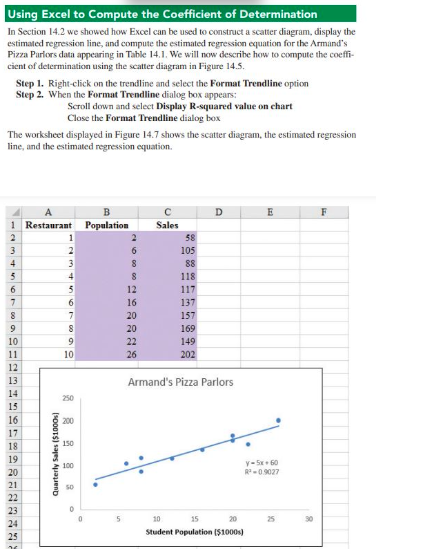
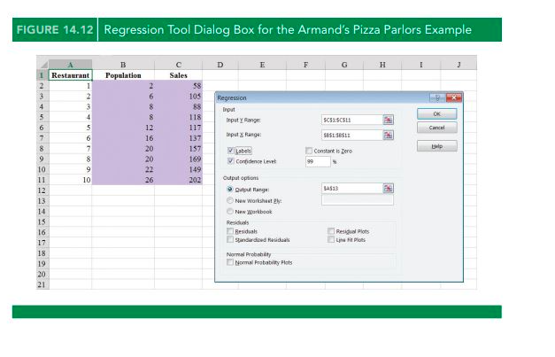
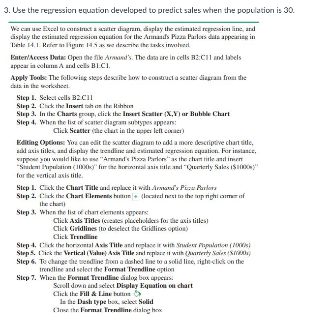
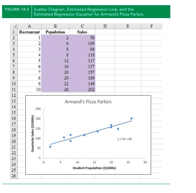
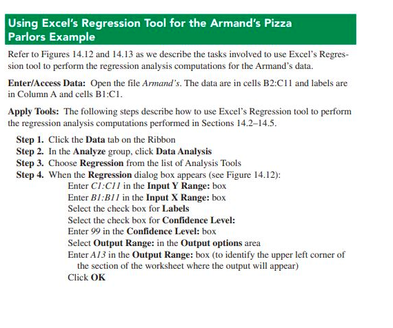
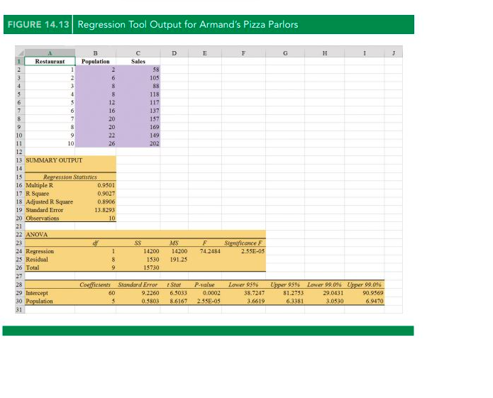
Please read chapter 14 and 15 Simple Linear Regression and Multiple Regression. Explore the DATA ANALYSIS (Excel) - Regression Analysis Tool. Refer to the results/answers presented in the book. To be submitted within the day. Less 5pts if not substantially completed and submitted within the day. No credit if submitted after May 27, 11:59 PM. Please copy the excel results and paste to word file and then convert to pdf file (File convention: SURNAME, First Name_Linear Regression Using Armand's xis file, please follow the Illustration presented in the reference book 1. Use Excel to develop a scatter diagram and to compute the least squares estimated regression equation and the coefficient of determination. (Refer to Figure 14.3 and Figure 14.4) 2. Use Excel's Regression Tool to answer the following questions. What is the estimated regression equation? Perform a t test and determine whether or not x and y are related. Use a = 0.01. Perform an F test and determine whether or not x and y are related. Use a = 0.01. Find and interpret the coefficient of determination.3. Use the regression equation developed to predict sales when the population is 30. We can use Excel to construct a scatter diagram, display the estimated regression line, and display the estimated regression equation for the Armand's Pizza Parlors data appearing in Table 14.1. Refer to Figure 14.5 as we describe the tasks involved. Enter/Access Data: Open the file Armand's. The data are in cells B2:C1 1 and labels appear in column A and cells BI:CI. Apply Tools: The following steps describe how to construct a scatter diagram from the data in the worksheet. Step 1. Select cells B2:ClI Step 2. Click the Insert tab on the Ribbon Step 3. In the Charts group, click the Insert Scatter (X,Y) or Bubble Chart Step 4. When the list of scatter diagram subtypes appears: Click Scatter (the chart in the upper left corner) Editing Options: You can edit the scatter diagram to add a more descriptive chart title, add axis titles, and display the trendline and estimated regression equation. For instance, suppose you would like to use "Armand's Pizza Parlors" as the chart title and insert "Student Population (1000s)" for the horizontal axis title and "Quarterly Sales ($1000s)" for the vertical axis title. Step 1. Click the Chart Title and replace it with Armand's Pizza Parlors Step 2. Click the Chart Elements button + (located next to the top right corner of the chart) Step 3. When the list of chart elements appears: Click Axis Titles (creates placeholders for the axis titles) Click Gridlines (to deselect the Gridlines option) Click Trendline Step 4. Click the horizontal Axis Title and replace it with Student Population (1000s) Step 5. Click the Vertical (Value) Axis Title and replace it with Quarterly Sales ($1000s) Step 6. To change the trendline from a dashed line to a solid line, right-click on the trendline and select the Format Trendline option Step 7. When the Format Trendline dialog box appears: Scroll down and select Display Equation on chart Click the Fill & Line button In the Dash type box, select Solid Close the Format Trendline dialog boxFIGURE 14.5 Scatter Diagram, Estimated Regression Line, and the Estimated Regression Equation for Armand's Pizza Parlors A B C D E F Restaurant Population Sales 58 105 8 88 118 12 117 16 137 20 157 20 169 22 149 10 26 202 Armand's Pizza Parlors 250 200 150 Quarterly Sales ($1000s) 100 y = 5x + 60 50 D 5 10 15 20 25 30 Student Population ($1000s)Using Excel to Compute the Coefficient of Determination In Section 14.2 we showed how Excel can be used to construct a scatter diagram, display the estimated regression line, and compute the estimated regression equation for the Armand's Pizza Parlors data appearing in Table 14.1. We will now describe how to compute the coeffi- cient of determination using the scatter diagram in Figure 14.5. Step 1. Right-click on the trendline and select the Format Trendline option Step 2. When the Format Trendline dialog box appears: Scroll down and select Display R-squared value on chart Close the Format Trendline dialog box The worksheet displayed in Figure 14.7 shows the scatter diagram, the estimated regression line, and the estimated regression equation. A B C D E F Restaurant Population Sales 58 6 105 8 88 118 12 117 16 137 20 157 20 169 10 22 149 26 202 Armand's Pizza Parlors 14 250 15 16 200 150 Quarterly Sales ($1000s) 100 Y = 5x +60 RT= 0.9027 50 5 10 15 20 25 30 Student Population ($1000s)Using Excel's Regression Tool for the Armand's Pizza Parlors Example Refer to Figures 14.12 and 14.13 as we describe the tasks involved to use Excel's Regres- sion tool to perform the regression analysis computations for the Armand's data. Enter/Access Data: Open the file Armand's. The data are in cells B2:C11 and labels are in Column A and cells BI:CI. Apply Tools: The following steps describe how to use Excel's Regression tool to perform the regression analysis computations performed in Sections 14.2-14.5. Step 1. Click the Data tab on the Ribbon Step 2. In the Analyze group, click Data Analysis Step 3. Choose Regression from the list of Analysis Tools Step 4. When the Regression dialog box appears (see Figure 14.12): Enter C/:C/ / in the Input Y Range: box Enter B/:B/ / in the Input X Range: box Select the check box for Labels Select the check box for Confidence Level: Enter 99 in the Confidence Level: box Select Output Range: in the Output options area Enter A/3 in the Output Range: box (to identify the upper left corner of the section of the worksheet where the output will appear) Click OKFIGURE 14.12 Regression Tool Dialog Box for the Armand's Pizza Parlors Example A B C D E F G H 1 Restaurant Population Sales 58 105 Regression Iput 118 InputY Fangs 117 Cancel 16 137 20 157 Labels Constant is Zero 20 159 Pi Confidence Level 21 149 10 26 202 Output opson Output Flange: New Worksheet Et. New Workbook 15 16 Residual peligun Plots 17 18 Normal Probebitty 19 Normal Probability Flats 20FIGURE 14.13 Regression Tool Output for Armand's Pizza Parlors B C D E F G H 1 J Restaurant Population Sales 58 105 118 12 117 16 137 20 137 20 169 10 21 149 10 26 202 13 SUMMARY OUTPUT 14 13 Repression Workfics 16 Multiple R 0.9501 17 R Square P.9017 18 Adjusted R Square 0.8906 19 Standard Error 13.8793 20 Choservations 10 21 22 ANOVA 23 F Stemricance F 24 Regression 14200 14200 74.2484 2.550-05 25 Residual 40 0 1530 191 25 26 Total 15730 27 28 Coefficients Standard Error Star P-value Lower 9596 Upper 9596 Lower 90.016 Upper 90.096 29 hilercept 60 9.2260 6.5033 0.0002 38.7247 81.2753 29.0431 90.9569 30 Population 0,5803 8.6167 2.45E-05 3.6619 6.3381 3,0530 6.9470 31MULTIPLE REGRESSION Using Butler File, Develop the Estimated Multiple Regression Equation using Excel's Regression Tool. Also, please present how you determined the results, example for coefficient determination R^2 = SSR/SST ; p value