Please show all matlab code -

lsdenoising.m is a vector of 1000 points that show the estimated signal - it's too long to post but this is what it looks like:

and it's defined like this

function xcor = lsdenoising

% denoising using least-squares

xcor= [-1.0814120288205518e-02

-4.1605052740093837e-02

3.2715248856760313e-03

etc etc - again it's too long to include the entire file but just use random numbers and show how it would be solved if the file were correct

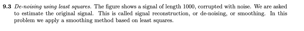
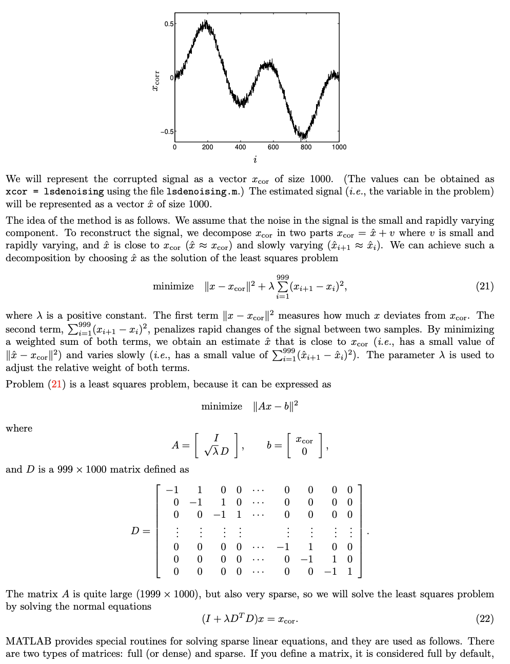
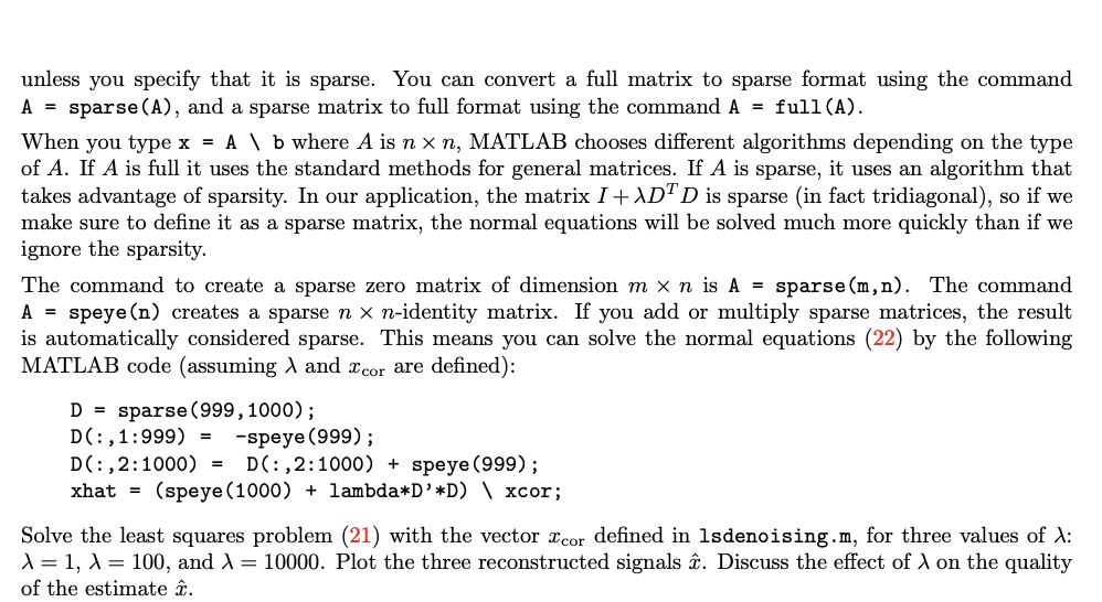
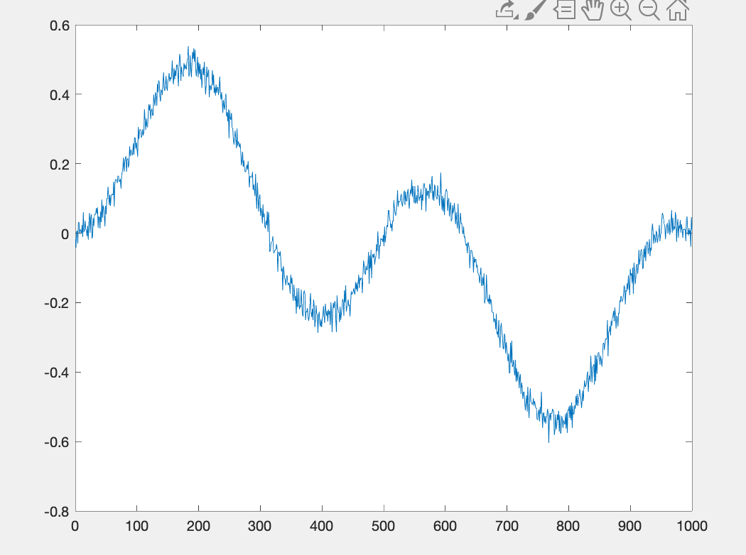
9.3 De-noising using least squares. The figure shows a signal of length 1000, corrupted with noise. We are asked to estimate the original signal. This is called signal reconstruction, or de-noising, or smoothing. In this problem we apply a smoothing method based on least squares. 0.51 corr 200 400 600 800 1000 We will represent the corrupted signal as a vector cor of size 1000. (The values can be obtained as xcor = lsdenoising using the file lsdenoising.m.) The estimated signal (i.e., the variable in the problem) will be represented as a vector of size 1000. The idea of the method is as follows. We assume that the noise in the signal is the small and rapidly varying component. To reconstruct the signal, we decompose cor in two parts cor = c + v where v is small and rapidly varying, and is close to Icor ( I cor) and slowly varying (li+1 = i). We can achieve such a decomposition by choosing as the solution of the least squares problem 999 minimize || 2 X cor ||2 + 1 (Xi+1 x;)?, (21) i=1 where is a positive constant. The first term ||X I cor ||2 measures how much x deviates from Icor. The second term, (Xi+1 - Xi), penalizes rapid changes of the signal between two samples. By minimizing a weighted sum of both terms, we obtain an estimate that is close to Xcor (i.e., has a small value of || - Icor ||2) and varies slowly i.e., has a small value of y(i+1 )). The parameter 1 is used to adjust the relative weight of both terms. Problem (21) is a least squares problem, because it can be expressed as minimize || Ax 6||2 where A= [vd] -=[ Sovt] 0 and D is a 999 x 1000 matrix defined as [ -1 1 0 0 ... -1 10 ... 0 0 -1 1 ... D= 1 : 0 0 0 0 ... 0 0 0 ... 0 0 0 ... 0 0 0 0 0 0 1 0 0 0 0 : 0 0 o o 1 0 -1 1 -1 0 0 1 -1 0 The matrix A is quite large (1999 x 1000), but also very sparse, so we will solve the least squares problem by solving the normal equations (I + XD+Dx = Xcor- (22) MATLAB provides special routines for solving sparse linear equations, and they are used as follows. There are two types of matrices: full (or dense) and sparse. If you define a matrix, it is considered full by default, unless you specify that it is sparse. You can convert a full matrix to sparse format using the command A = sparse(A), and a sparse matrix to full format using the command A = full(A). When you type x = A \ b where A is n xn, MATLAB chooses different algorithms depending on the type of A. If A is full it uses the standard methods for general matrices. If A is sparse, it uses an algorithm that takes advantage of sparsity. In our application, the matrix I + ADD is sparse in fact tridiagonal), so if we make sure to define it as a sparse matrix, the normal equations will be solved much more quickly than if we ignore the sparsity. The command to create a sparse zero matrix of dimension m x n is A = sparse(m,n). The command A = speye(n) creates a sparse n x n-identity matrix. If you add or multiply sparse matrices, the result is automatically considered sparse. This means you can solve the normal equations (22) by the following MATLAB code (assuming and Xcor are defined): D = sparse (999, 1000); D(:,1:999) = -speye (999); D(:,2:1000) = D(:,2:1000) + speye (999); xhat = (speye (1000) + lambda*D'*D) | xcor; Solve the least squares problem (21) with the vector Icor defined in lsdenoising.m, for three values of 1: 1=1, = 100, and = 10000. Plot the three reconstructed signals . Discuss the effect of on the quality of the estimate o 0.6 0.4 no -0.4 -0.6 -0.8 0 100 200 300 400 500 600 700 800 900 1000 9.3 De-noising using least squares. The figure shows a signal of length 1000, corrupted with noise. We are asked to estimate the original signal. This is called signal reconstruction, or de-noising, or smoothing. In this problem we apply a smoothing method based on least squares. 0.51 corr 200 400 600 800 1000 We will represent the corrupted signal as a vector cor of size 1000. (The values can be obtained as xcor = lsdenoising using the file lsdenoising.m.) The estimated signal (i.e., the variable in the problem) will be represented as a vector of size 1000. The idea of the method is as follows. We assume that the noise in the signal is the small and rapidly varying component. To reconstruct the signal, we decompose cor in two parts cor = c + v where v is small and rapidly varying, and is close to Icor ( I cor) and slowly varying (li+1 = i). We can achieve such a decomposition by choosing as the solution of the least squares problem 999 minimize || 2 X cor ||2 + 1 (Xi+1 x;)?, (21) i=1 where is a positive constant. The first term ||X I cor ||2 measures how much x deviates from Icor. The second term, (Xi+1 - Xi), penalizes rapid changes of the signal between two samples. By minimizing a weighted sum of both terms, we obtain an estimate that is close to Xcor (i.e., has a small value of || - Icor ||2) and varies slowly i.e., has a small value of y(i+1 )). The parameter 1 is used to adjust the relative weight of both terms. Problem (21) is a least squares problem, because it can be expressed as minimize || Ax 6||2 where A= [vd] -=[ Sovt] 0 and D is a 999 x 1000 matrix defined as [ -1 1 0 0 ... -1 10 ... 0 0 -1 1 ... D= 1 : 0 0 0 0 ... 0 0 0 ... 0 0 0 ... 0 0 0 0 0 0 1 0 0 0 0 : 0 0 o o 1 0 -1 1 -1 0 0 1 -1 0 The matrix A is quite large (1999 x 1000), but also very sparse, so we will solve the least squares problem by solving the normal equations (I + XD+Dx = Xcor- (22) MATLAB provides special routines for solving sparse linear equations, and they are used as follows. There are two types of matrices: full (or dense) and sparse. If you define a matrix, it is considered full by default, unless you specify that it is sparse. You can convert a full matrix to sparse format using the command A = sparse(A), and a sparse matrix to full format using the command A = full(A). When you type x = A \ b where A is n xn, MATLAB chooses different algorithms depending on the type of A. If A is full it uses the standard methods for general matrices. If A is sparse, it uses an algorithm that takes advantage of sparsity. In our application, the matrix I + ADD is sparse in fact tridiagonal), so if we make sure to define it as a sparse matrix, the normal equations will be solved much more quickly than if we ignore the sparsity. The command to create a sparse zero matrix of dimension m x n is A = sparse(m,n). The command A = speye(n) creates a sparse n x n-identity matrix. If you add or multiply sparse matrices, the result is automatically considered sparse. This means you can solve the normal equations (22) by the following MATLAB code (assuming and Xcor are defined): D = sparse (999, 1000); D(:,1:999) = -speye (999); D(:,2:1000) = D(:,2:1000) + speye (999); xhat = (speye (1000) + lambda*D'*D) | xcor; Solve the least squares problem (21) with the vector Icor defined in lsdenoising.m, for three values of 1: 1=1, = 100, and = 10000. Plot the three reconstructed signals . Discuss the effect of on the quality of the estimate o 0.6 0.4 no -0.4 -0.6 -0.8 0 100 200 300 400 500 600 700 800 900 1000