Please Show the MATLAB code for this. Thank you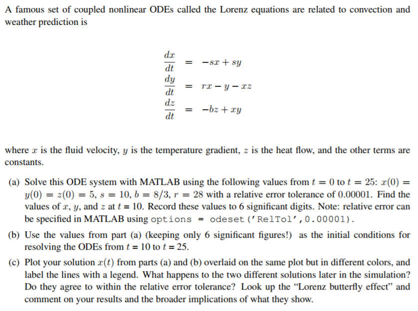

A famous set of coupled nonlinear ODEs called the Lorenz equations are related to convection and weather prediction is da -sx + sy r-y-2 -bz + xy = dt dt dt = where is the fluid velocity, y is the temperature gradient, z is the heat flow, and the other terms are constants (a) Solve this ODE system with MATLAB using the following values from t = 0 to t = 25: 2(0) y(0) = z(0) = 5, s-10, b = 8/3, r = 28 with a relative error tolerance of 0.00001. Find the values of x, y, and z at t10. Record these values to 6 significant digits. Note: relative error can be specified in MATLAB using options = odeset ("RelTol. 0 . O0001). (b) Use the values from part (a) (keeping only 6 significant figures!) as the initial conditions for resolving the ODEs from t 10 to t = 25. (c) Plot your solution (t) from parts (a) and (b) overlaid on the same plot but in different colors, and label the lines with a legend. What happens to the two different solutions later in the simulation? Do they agree to within the relative error tolerance? Look up the "Lorenz butterfly effect" and comment on your results and the broader implications of what they show. A famous set of coupled nonlinear ODEs called the Lorenz equations are related to convection and weather prediction is da -sx + sy r-y-2 -bz + xy = dt dt dt = where is the fluid velocity, y is the temperature gradient, z is the heat flow, and the other terms are constants (a) Solve this ODE system with MATLAB using the following values from t = 0 to t = 25: 2(0) y(0) = z(0) = 5, s-10, b = 8/3, r = 28 with a relative error tolerance of 0.00001. Find the values of x, y, and z at t10. Record these values to 6 significant digits. Note: relative error can be specified in MATLAB using options = odeset ("RelTol. 0 . O0001). (b) Use the values from part (a) (keeping only 6 significant figures!) as the initial conditions for resolving the ODEs from t 10 to t = 25. (c) Plot your solution (t) from parts (a) and (b) overlaid on the same plot but in different colors, and label the lines with a legend. What happens to the two different solutions later in the simulation? Do they agree to within the relative error tolerance? Look up the "Lorenz butterfly effect" and comment on your results and the broader implications of what they show